Physics of Musical Instruments Project Plan

Physics of Musical Instruments Project Plan

Greg Cristina, Teddy Stanescu


Objective:  Explore the physics behind the sound of different musical instruments; vibrations through different mediums and the frequencies they create. We will be looking to experiment with these three musical instruments:


  1. Guitar (a plucked string)
  2. Piano (a hammered string)
  3. Drum (a hammered membrane)


Chapter/Section(s) of Focus: We will focus on theory and use equations from Chapter 11 in the class text (Giordano), specifically sections 11.1, 11.2, and 11.4.


Overview: We want to model each of these 3 instruments in Matlab, using the computational methods and equations provided in the text.  These models will consist of the physical behavior of the instruments, such as (x,y,z) displacement of a string/membrane at a given time t and the frequencies/harmonics (overtones) they produce given specified initial conditions.  From here, we will take advantage of Matlab’s ability to read and extrapolate data from audio files by mimicking our theoretical scenarios modeled in Matlab as a physical test, using the actual instruments, keeping as many initial parameters as possible constant.  We will record the sound produced by the instruments using a microphone and recording software (audacity/reaper), import to Matlab, and compare the recorded data to the data calculated through the computational methods.


Experimentation:  For the guitar string, we will pluck the string at different distances from the bridge.  For the piano string, we will strike the string with different strength forces from the hammer.  These changes in how the instrument is played are shown in the text to yield different frequencies and harmonics, and we will further investigate this phenomenon.  The drum will be the biggest challenge to experiment with because there is no direct example in the text.  However, it covers many methods that we will modify and test such as relating the force of a guitar or piano string on the soundboard to the frequency it produces.  Also, the text has a banjo example of how a wave on a string affects a membrane and the frequencies they produce, which is similar to the two heads of a drum interacting with each other to produce a sound.  Using knowledge gained from experimenting with the guitar and piano strings, we will investigate drum membrane physics and attempt to model in Matlab, if model is successful, a recording with be made and compared.


Sources used (as of now):

Computational Physics, Nicholas Giordano

-more to come if necessary


Timeline:

Week 1 – Model guitar string in Matlab, and test at different distances from bridge.

Week 2 – Model piano string in Matlab, and test different hammer forces

Week 3 – Record guitar and piano string, analyze and compare with Matlab calculated data

Week 4 – Drum experimentation

Week 5 – Organize data in a presentable manner, fix any errors in data analysis

John Loree Project Outline

The goal of this project is to extract 2 relevant measures stemming from an EMG or nerve signal, the peak cycle amplitude and cycle duration. These two measures as demonstrated in several academic papers in a variety of model organisms, are the measures most consistently correlating with a muscle response. An idealized nerve spike train signal appears as repeating spikes, whose amplitudes and frequencies vary according to the action at hand. However, this method has several issues with both execution and correlating to the physical model. Primarily, depending on the scenario at hand, there will be constant low level nerve activity corresponding to maintaining a given muscular contraction, this activity is extremely difficult to distinguish from noise.

The relevant measure will be quasi-linked in the code, with the program measuring nothing, peak amplitude, or amplitude and cycle duration depending on the magnitude of the signal from the EMG. However, prior to any signal extraction, the program will run a Fourier transform (due to software, hardware  and time restrictions, this iteration will likely store data in bins and process after each bin, as opposed to continuous measurement), excise the largest and most common noise signals (such as 60Hz noise emanated by  many electronic devices), and transform the spectrum back as a rectified signal. The system will not update (essentially being in a resting state), when there are no peaks above a noise threshold for a given duration. This  first threshold, determined by measuring the mean peak magnitude of noise registered by the EMG that is not connected to a live test subject will provide a lower limit on the kinds of information that the program will save. Above this first threshold, the program will record the peak amplitudes of the EMG signal. This can be used to keep the robotic agent at some non-resting state, without any motion. A second threshold, determined by the difference of magnitude between 2 measured peaks, will incite contraction in the arm. Once this threshold is passed, the program will measure all peaks for the cycle, and the the cycle duration (start and finish determined by the difference between each contracting peak and the last pre-contraction peak). The cycle duration will control the length of the contraction as determined by a scale elsewhere in the project, and the highest peak will be used to set the speed of the robotic arm’s motion.

Each signal will correspond to a single robotic degree of freedom, such that this program will be repeated uniquely for each EMG channel. A major limitation at this initial stage of design is available processing time, as the time required to process each signal will likely exceed the time that the biological agent would execute the same motion. As such, this initial setup will have signals taken at a different time than processing. This iteration will be written in Matlab, although later versions of the code will likely be run elsewhere.

Timeline:

Week 1: Execute background research, create an architecture on paper to use as a blueprint for the actual program

Week 2: Write the code for the Fourier transform, bin size to be determined later, harvest the noise signal and find the lower threshold for the data acquisition program

Week 3: Write the code to gather the relevant signals and set the thresholds and bin sizes depending on processing time.

Week 4: Finish writing/modifying code, prepare presentation and write up report for the project.

Sources:

TBD (There are several from the thesis list, I just have to select which ones I am going to use and possibly gather a few others)

Project Plan Celestial Mechanics: Precession and Kirkwood Gaps

The goal of this project is to investigate two problems in celestial mechanics for which a computational solution is quite valuable: the precession of the perihelion of Mercury and Kirkwood gaps, both found in Chapter 4 of Computational Physics by Giordano and Nakanishi. In the case of Mercury, the precession can be calculated analytically thanks to general relativity, but a computational solution is easier to obtain. Giordano and Nakanishi describe the process of obtaining the rate of precession, keeping in mind that this variable must be adjusted for practical computation times (that is, not 230,000 years), using the force law predicted by general relativity:
F_G ≈ (G M_S M_M)/r^2 (1+a/r^2 ),
Where M_M≡mass of Mercury, M_S≡mass of Sun ,a ≈1.1 ×〖10〗^(-8) 〖AU〗^2.
Part of the project will be to compare different computational methods for analyzing this procession, particularly the Euler-Cromer method and Runge-Kutta (which uses the Euler-Cromer method to update its values). Using a two-body system simulation, the value for rate of procession can be found by varying until it matches expected, observed rates.

The second computational problem covered is one for which an analytical solution is difficult, as the system is considered chaotic. In our solar system there are certain “gaps” in orbital radii from the Sun at which there are far fewer asteroids. Numerically it can be found that these gaps occur at certain resonances with Jupiter’s orbit, such as 2/1, 5/2, 7/3, etc. Running a simulation to find Kirkwood gaps and investigate asteroids’ paths near these gaps first involves construction of a multi-body model, at least a two-body system for the Jupiter and Sun, and for more accuracy (if time permits) a three-body system along with the Earth. Luckily the magnitude comparison between Jupiter and an asteroid makes their mass insignificant, meaning their gravitational force can be excluded from the simulation without much effect on accuracy of the program. An analysis of the asteroid’s orbits will also naturally include a discussion of chaos, described in Chapter 3 of Giordano and Nakanishi.

Timeline:
Week 1: Continue background research on physics and computational methods of analysis, write code for precession of perihelion of Mercury, begin (and hopefully finish) writing code for 2- or 3-body system in Kirkwood problem
Week 2: Adjust solar system model to include simulations of asteroids, their paths/orbits, finish all code, begin gathering data.
Week 3: Finish gathering data, finish all research, comparison to actual observed/computer values from literature sources.
Week 4: Finish data analysis, write-up for project, prepare presentation.

Sources:
Computational Physics, Giordano and Nakanishi, Chapters 3 & 4.
Mercury’s Perihelion from Le Verrier to Einstein, N.T. Roseveare.
Chaotic Dynamics in the Solar System, J. Wisdom.

3-Body Celestial Mechanics Project Plan (Nadav and Matteo)

Purpose and Goals

One purpose of this course is to explore the use of computational methods to find solutions to otherwise difficult analytical problems. The 3-body system is a prominent example. It is relatively straightforward to solve the equations of motion of a 2-body problem analytically, but far more difficult to do so for 3 bodies. The introduction of computational methods have allowed for fairly straightforward ways of analyzing 3-body motion.

A prominent example is that of the Sun, the Earth, and Jupiter, bound by the force of gravity. Since Jupiter is about 0.1% of the solar mass, it is the next biggest influence on Earth’s orbit in the Solar system. Using computational methods to analyze Jupiter’s effect would be far more efficient. We seek to create a model of the orbits of the Earth and Jupiter bound to the sun–and interacting with each other–via the inverse square law of gravity.

For this project we plan to make use of sections 4.1 and 4.4 in Giordano’s book. 4.1 outlines a method for calculating the motion of a planet orbiting the sun, whereas 4.4 opens the model to include Jupiter. The program will generate position data for each planet given their acceleration due to gravity, using the Euler-Cromer Method to approximate each new position based on this acceleration. We will start with a simplified model, with the Sun fixed to the origin, then graduate to a true 3-body model, where the origin would be fixed at the system’s center of mass.

Physics

We start with Newton’s Law of Gravitation, where Ms is the solar mass, Mp is the planet Mass, Fp is the gravitational force experience by the planet due to the Sun, and G is the gravitational constant:

Fp=G*Ms*Mp/r^2

Solving for acceleration (given Newton’s 2nd Law: Fp=Mp*a), or d^2x/dt^2:

a=G*Ms/r^2

This solution for acceleration is a second order differential equation, appropriate for use with the Euler Cromer Method.

Foundational Code (Routines provided in Giordano)

Planets: A routine to model the orbit of a planet around the sun as described by the inverse square law of gravitational force, with the sun at the origin. The Euler-Cromer method is used to approximate position. The Euler Method by itself would not be sufficient, as with all oscillatory motion it would introduce energy into the system and the planet would move away from the Sun. The Euler-Cromer Method guarantees a conservation of energy over one orbit.

Jupiter-Earth: Expands the above system to model Jupiter and Earth orbiting the sun. This method will also use the Euler-Cromer method for the same reasons. The suns mass will affect the orbits of the other two planets but the sun itself will sit at the origin of the system and not move.

True 3-body: This model is similar to the Jupiter-Earth model but instead uses the center of mass of the system as the origin. This model will be used when we are altering the mass of jupiter to be close to that of the sun, therefore causing changing orbits for each planet in the system. In this case, we want the sun to be able to move to better describe the full motion.

Initial Resources

http://astro.geo.tu-dresden.de/~klioner/celmech.pdf

http://arxiv.org/pdf/astro-ph/0411043v1.pdf

http://www.iumj.indiana.edu/docs/27030/27030.asp

Computational Physics, Giordano and Nakanishi. Sections 4.1 and 4.4.

Timeline

Week 1 (4/6-4/12)

During the first week we hope to work on organizing sources and solidifying understanding of background materials and physics. We will also use this week to read the Giordano text to begin understanding the setup of the MATLAB routines. We will begin writing the code for the Planets routine. This routine does not directly inform the 3-body problem but is the foundational code for the project. For the entire first week we will split the workload together since this work constitutes the base understanding of our project.

Week 2 (4/13-4/19)

Since the Planets routine should be well defined and operational by this week, we will use this time to finish off the other routines. This should be manageable since both the Jupiter-Earth and True 3-body routines are derivations of the Planets routine. Nadav will work on the Jupiter-Earth model while Matteo tackles the True 3-Body routine. This week will mostly be coding based, as we hope have all models complete by this time.

Week 3 (4/20-4/26)

By now, all routines should be complete. We will use this week to explore the implications of our models. This exploration will consist of multiple demonstrations of the effects of the changed mass of Jupiter on the system and will also include qualitative conclusions. We will also begin to work on writing up our results, with each of us taking charge of specific simulations.

Week 4 (4/27-5/3)

This final week will consist of finishing up our written results and finalizing the report. We will also leave space here for potential further exploration of our system, given appropriate time. Possible extensions include adding in another body to the system or analyzing in more detail the stability of orbits (Section 4.2, Giordano).

Project Plan: Drunken MATLAB Journey

Through random system analysis, I would like to determine both a trend for 2D motion between 2 locations and how altering specific real world variables can change this trend. I will be using Chapter 7 of the class text the most for the basic bulk of the code. However, I will be developing novel aspects for my code in order to simulate certain variables within the random journey.

This epic journey will be through the weary eyes of a Vassar student struggling and stumbling (strumbling, if you will) their way back from a long and alcohol filled night. We find this student past inebriation and past wasted: at this point, the poor soul is taking random steps in random 90 degree turns back to their room. They even fall down from time to time. However, there is hope yet! They have a friend with them that will guide them back to their dorm with a gentle push from time to time. How long will it take them to make it back?

The random variables listed above (and I will probably find some more) will be simulated by additional conditions in the MATLAB code and represent real and mathematic aspects of random motion. I will analyze their effects and relative weights of each via multiple graphs that will attempt to find a trend or average number of steps for a certain distance. I would then like to increase the distance gradually in order to find an expression for displacement traveled and the number of steps required.

I would like to present my data as scatterplots of steps required. By adding additional variables during the walk, I can compare their individual effects. In addition, I can watch the effects the relative weights each variable has on the outcome. For example, does a higher rate of falling down change the outcome more than less drift induced from the friend? Toying with relative weights can also make the journey more realistic.

This project allows me to use statistical analysis and probability to map the path of an independent data point with variables imposed on it. This introduces a lot of variance in the data and my largest stumbling block (get it?) will be extracting concrete data from this. Data might also be difficult to extract with pure random motion at long distances. This project also leaves different relationships between variables wide open so I can qualitatively compare variables if concrete data is weak.


Week 1

Writing the bulk of the code and determining whether there is a trend without drift.

Week 2

Implementing additional variables and watching their affect on steps required

Week 3

Data compilation and figure creation

Week 4

Hopefully I’m done around here but if not, I might add another variable to the mix and see how it affects the steps required to reach the destination. Data compilation might spill over into this week too.

Orbital Motion Simulation – Frye and Gittins


We plan on modeling objects in orbital motion, namely the sun and earth, the earth and moon, the three together, and finally an orbit of two large-massed bodies, such as the sun and another star.

The programming steps we need to take are straightforward in theory. We have already settled on using the Euler-Cromer method on MatLab to simulate the motion. We have access and prior knowledge of Newton’s laws and Kepler’s laws of motion, as shown below.  The potentially difficult part will be writing a program that will be able to track the motion of several bodies simultaneously, with the capability of visualization, such as a moving graphic.


(1)   \begin{equation*} \ F_{G}=\frac{GM_{S}M_{E}}{r^{^{2}}} \end{equation*}


where Ms is the mass of the sun and Me is the mass of the earth.


Kepler’s Laws:

  • All planets move in elliptical orbits with the Sun at one focus.
  • The line joining a planet to the Sun sweeps out equal areas in equal times.
  • If T is the period and a the semimajor axis of the orbit, then T^2/a^3

(2)   \begin{equation*} \frac {d^{2}x}{dt^{2}} = \frac {F_{Gx}}{M_{E}} \end{equation*}

(3)   \begin{equation*} \frac {d^{2}y}{dt^{2}} = \frac {F_{Gy}}{M_{E}} \end{equation*}


from which we can derive the equation:

(4)   \begin{equation*} \ F_{Gx}=-\frac{GM_{S}M_{E}}{r^{2}}\cos{\theta}=-\frac{GM_{S}M_{E}x}{r^{3}} \end{equation*}

for the x-direction. A similar equation can be found for the y-direction. For the equations of motion that will be put into the Euler-Cromer program, we will use equations similar to those derived in Giordano.


(5)   \begin{equation*} \ v_{x,i+1}=v_{x,i}- \frac{4\pi^{2}x_{i}}{r_{i}^{3}}\Delta{t} \end{equation*}

(6)   \begin{equation*} \ x_{i+1}=x_{i}+v_{x,i+1}\Delta{t} \end{equation*}

(7)   \begin{equation*} \ v_{y,i+1}=v_{y,i}- \frac{4\pi^{2}y_{i}}{r_{i}^{3}}\Delta{t} \end{equation*}

(8)   \begin{equation*} \ y_{i+1}=y_{i}+v_{y,i+1}\Delta{t} \end{equation*}


For preliminary data, we hope to have a primitive program that has the capability of simulating a simple Earth-Sun orbit, assuming that the Sun is so massive (compared to Earth) that it does not move. We hope to have an appropriate visualisation, a moving plot, to apply to the data. At this time we will need to heavily research the physics of the situation, including providing details of what is physically incorrect about our simulation and the amount of error these details create. The defense of this simulation, including pros and cons of the Euler-Cromer method in this case, will be in the preliminary data.

The second goal is to make the system more complicated, either adding the moon or another planet to the existing system. As in the first set of data, we will need to analyze it for flaws. We anticipate this to be the most difficult programming challenge, as there are three systems moving simultaneously, and also the most complex error analysis.

Screen Shot 2015-04-01 at 12.10.11 AM

Finally, we plan to model a system in which each mass is in motion, for example, two large suns or a star and a large planet.  At this point, we will be fairly comfortable with the Euler-Cromer method applied to this system. Here, we will truly analyze the flaws with the method and compare and contrast these flaws, and its strengths, with other methods we have learned in class. This will also provide insight into our previous simulations and their errors, as the sun is not un-moving as we assume previously.

two massiv

We hope the final program will appear similar to the ones shown in Giordano and the exploration of orbits done by Moler.


Timeline:

Week 1: Research more equations and pseudo codes that relate to our simulation.

Week 2: Write a primitive program to simulate the earth and the sun orbit. Calculate error.

Week 3: Finish Earth-Sun simulation. Begin writing program for Moon-Earth-Sun by working with program from Week 2. Begin writing primitive program for two massive planets or stars.

Week 4: Finish program for two massive planets or stars. Calculate error. Troubleshoot Moon-Earth-Sun program.

Week 5: Finish all programs and prepare for presentations.


Resources

  1. Giordano. Computational Physics, 2006.
  2. Moler, Cleve. “Orbits,” MathWorks Inc, 2011.

Physics of Baroque Keyboard Instruments: Project Plan – Kachelein

Introduction

– In chapter 6 of the class text, we were first introduced to the motions of waves on strings, even modeling their motion in a few simple cases. In chapter 11, the physics of musical instruments is explored. The guitar and the piano are featured prominently in this chapter, as they have relatively simple mechanics and are stringed, hence the framework for exploring their behavior has been established. Other instruments, each with different physical characteristics, can also be modeled. The goal of my project is to start with information in chapter 11 and build full, working models of the harpsichord, clavichord and, hopefully, the pipe organ, three instruments with which I am very familiar. The final aim of the project is to compare computed data with actual signals from the instruments in question, verifying (or nullifying) the computational models.

Methods

– MATLAB will, of course, be used as the primary, if not sole, computational tool (if a difficult differential equation needs to be solved, Mathematica may be invoked). For the harpsichord, a model for the plucking force will need to be built (harpsichord strings are plucked, rather than struck like those of a piano). Though plucked strings are already discussed in the guitar sub-chapter, I feel that a more complicated but realistic model can be built (for example, by considering the effect of the plectra as the string slides off of it). The string’s motion will be governed, naturally, by the wave equation:

which is computationally realized by eq. 6.6:

– The clavichord is also a string instrument which has a striking mechanism like that of the piano, but which is physically much different. In particular, the forcing site is also a boundary of the string, so a radically different model from that of the piano/harpsichord may or may not need to be used.

– If the organ proves feasible after addressing the instruments above, I will attempt to model at least one type of pipe and at most two types (round metal and square wooden pipes). Part of chapter 11 addresses a one dimensional pipe, and the methods are claimed to be easily extendable to three dimensions using coupled partial differential equations. For the one dimensional case, we have pressure, p, and velocity, v, in air of density ρ and sound speed c given by:

which has a numerical form given by equation 11.37 in the book:

where Z is acoustic impedance, the correct value of which will be of particular importance (material dependent).

– The experimental portion of the project is not yet laid out. I may request assistance from Professor Bradley in taking and analyzing acoustic signals from the aforementioned instruments. Regardless, I intend to compare the Fourier transforms of actual signals to the computed transforms in order to see if the peak frequencies match.

Time Line

– Week 1: Practice by completing a few problems from chapter 11.

– Week 2: Build a working model for the harpsichord, as complete as the piano model in the book, and take data. Begin work on clavichord model.

– Week 3: Complete clavichord model. Begin organ model.

– Week 4: Complete organ model. Record real instruments to compare to models.

– Week 5: Compare experimental data to models. Allow time for write up and possible revision of models.

– Week 6: Further time, submit Wednesday.

Resources:

– Giordano N J, Nakanishi H. “Computational Physics, 2nd Edition.” 2005. Addison-Wesley. ISBN-10: 0131469908.

– MATLAB R2014b by MathWorks®

Project Plan Monte Carlo Simulation Financial Applications

The first objective of our project is to use MatLab to provide simple examples of how the Monte Carlo method can be used. To do this I will create a simple program that shows the distribution of numbers of a six-sided die land on when randomly thrown for a specific number of iterations. To do this I will use the basic method of the Monte Carlo method provided by our textbook Computational Physics by Nicholas J. Girodano and Hisao Nakanishi. The second program I will create will demonstrate how the Monte Carlo method can be used to find the moment of inertia for an object with a range of different measurements for different parameters. Finally the third simple program I will create will be using the Monte Carlo method to find how much money someone needs to be invested into a stock or portfolio of stocks to retire at certain age. All these simple programs use the concept of normal or lognormal distribution and take advantage of MatLab’s built in random number generator. With these simulations we will discuss how central limit theory provides a basis for the Monte Carlo method being an acceptable

The second goal of our project, Elias Kim and I will both attempt to use the Monte Carlo algorithm for the Ising model on an L x L square lattice, separately. The Ising model is an integral part of physics because it helps describe how neighboring atoms and their electron magnetic spins interact with one another and have the ability to change the neighboring electrons spin. In addition the Ising model is used to explain ferromagnetic interaction but its influence has extended into the world of thermodynamics as well. Elias and I will then join together to compare our answers to make sure we got similar solutions.

The final objective of our project, Elias and I will team up and use our knowledge of the Monte Carlo method and Ising model to tackle financial problems. The Ising model can be used to exam the volatility of a stock or portfolio and the risk associated with it. In the world of finance, volatility is defined as a statistical measure of the dispersion of returns for a given security or market index, this can be simply calculated with the standard deviation of returns from that same security or market index. Many factors that previously were thought as random actually alter the volatility of an asset, which is what Elias Kim, and I intend to investigate.


Timeline:

Week of April 6th : Acquire basic knowledge of Monte Carlo simulation and relevant equations and concepts. Continue researching about the Ising Model and various financial principles.

Week of April 13th : Create the three basic Monte Carlo simulations described in the General Plan, and begin to work on the simple Ising Model described in Computational Physics.

Week of April 20th :Finish the simple Ising Model, and compare results to Elias’ findings . Continue researching the Ising Model and its applications to the financial world.

Week of April 27th: Begin working on the applying the Ising Model to a financial problem. Continue researching on the Ising Model and its applications to finance.

Week of May 4th : Finish the collaboration with Elias and get ready for project presentations.

References:

1. Monte Carlo Techniques G. Cowan (RHUL).

2. Probability Review and Overview of Monte Carlo Martin Haugh

3. http://www.excelfunctions.net/Excel-Norminv-Function.html ExcelNet

4. Ising Model in Finance Pavel Dvoˇr´ak

5. Physics and Financial Economics (1776-2014): Puzzles, Ising and Agent-Based models

D. Sornette (ETH Zurich)

6. Phase transition in an Ising economy Miloš Borovšak

7. Statistical physics of social dynamics Claudio Castellano, Santo Fortunato, Vittorio Loreto

8. Computational Physics Nicholas J. Girodano, Hisao Nakanishi

Project Plan: Monte Carlo Method and its applications in Finance

Theoretical Motivation:

During the final stages of the Manhattan Project, Stanislaw Ulam and John Von Neumann developed the Monte Carlo method in order to calculate on average how long it would take for a neutron to collide with the nucleus of an atom when projected into a given substance. Named after the famous Monaco casino, Monte Carlo methods are often used to describe systems that have a set range of inputs and parameters, the specifics of which are unknown. The method inputs random or pseudo-random values into the system over and over again to see if a certain trend emerges when certain combinations of values are chosen. Often, Monte Carlo methods are used to simulate systems in physics that have many coupled degrees of freedom, such as radiation and fluid dynamics. However, many social scientists have since begun to use Monte Carlo simulations to predict the ways that certain trends develop, particularly in the world of finance and economics.

The Ising model emerged from the study of ferromagnetism, providing a way to study the interactions between adjacent atoms with discrete magnetic spin numbers. Since each spin influences its surrounding neighbors, these systems are modeled by creating a grid of cells that influence the cells around it based on a specific set of laws or equations. In the context of physics, the Ising model has since expanded from the field of ferromagnetism into thermodynamic phase transitions and other related fields. Like the Monte Carlo method, it has also been commandeered by the finance community to map the progress of interrelated variables and actors in an economic system. It does so by defining a set of actors governed by mutual economic and financial laws.

Finally, in the world of finance, volatility refers to the way that a financial instrument’s price changes over time. Many traditional models of volatility follow a deterministic approach in which the price of a financial security (any type of financial asset) has a constant volatility over time. However, these models often fail because the volatility of any given security is in reality stochastic over time and evolves due to the contributions of many factors, some of which cannot be seen directly. To account for this stochastic volatility when determining the price of financial assets, economists have often turned to Monte Carlo methods and the Ising model to predict the way interrelated, seemingly random factors evolve over time. Adam Warner and I plan to gain a preliminary understanding of the way that these methods transfer from physics to the world of finance.

Description:

I will begin my study by using MatLab to write very basic examples of both an Ising system and an independent Monte Carlo method, starting with the discussion in Giordano’s computational physics. I will then use a Monte Carlo simulation to solve a more rigorous physics problem, concerning the emission of radiation from an atom. This process is stochastic in nature, so I believe it will be a good precursor to looking at the kind of method necessary to solve a financial volatility problem. I will then attempt to model the volatility of a derivative security, a financial asset that depends on the prices of other more basic assets. Finally, if time allows, Adam and I will work together to develop an Ising model that describes an economic system.

Timeline:

Week 1 (4/6-4/12)

I will finish my research on the basic principles of the Ising Model, Monte Carlo Methods, and Volatility. I would like to have a comprehensive list of papers to reference and be ready to start working in MatLab.

Week 2 (4/13-4/19)

At this point, I will start to work on my models for the basic Monte Carlo and Ising problems. I do not think that these will be too rigorous and I hope to be able to display these in my first preliminary results report. I will need to figure out the kind of notation to use for this sort of computation.

Week 3 (4/20-4/26)

By then, I should be ready to start my model of atomic radiation. This will help me get a good grasp on how to approach a stochastic system in MatLab and should be an example of some pretty interesting physics concepts. I hope to get this into my preliminary results as well, but am less certain.

Week 4 (4/27-5/3)

Now, I will attack the meat of my project. I will use all of the concepts I have worked with up to this point to model the stochastic evolution of the volatility of derivative security.

Week 5 (5/4-5/10)

This week I should be able to finish the model described previously. If all goes according to plan, I will have time to work with Adam on characterizing how an Ising model would be able to describe the evolution of interconnected securities and the decisions made to give them prices.

Sources:
1. Computational Physics, Giordano and Nakanishi
2. Physics and Financial Economics (1776-2014): Puzzles, Ising and Agent-Based models
D. Sornette (ETH Zurich)
3. University of Virginia: Introduction to Atomic Simulations, Leonid Zhigilei
4. Probability Review and Overview of Monte Carlo, Martin Haugh
5. Monte Carlo Methods for Security Pricing, Phelim Boyle, Mark Boardie, Paul Glasserman
6. Monte Carlo simulation of the atomic master equation for spontaneous emission
R. Dum, P. Zoller, and H. Ritsch

Precession of Mercurian Planets: Project Plan

Goals:

For my computational physics project I would like to investigate the relationship between the precession and the eccentricity of a planet’s orbit due to general relativity as detailed in chapter 4, section 3 of Computational Physics, by Nicholas J. Giordano and Hisao Nakanishi. The rate of precession examined in this project will only be that which is caused by the general relativistic effect of the model planet’s host star.

Week 1: Preliminary Results

As a check to make sure my code will run correctly, I will first model the precession of Mercury’s orbit as caused by the Sun. I must first write a code that will model the movement of a Mercury through it’s orbit according to Kepler’s laws. The force law predicted by General Relativity is given by:

 Fg=\frac{GM_{s}M_{m}}{r^{2}}(1+\frac{\alpha}{r^{2}})

where G is the Gravitational constant of the universe, Ms is the mass of the Sun, Mm is the mass of Mercury, and a Constant*α gives the rate of precession for the orbit. For the case of Mercury,  \alpha=1.1*10^{-8} AU^{2} .

Applying the Euler-Chromer method to the above equation to approximate the x and y velocities and positions of the planet as it travels throughout its orbit yields:

 V_{x,i+1}= V_{x,i}-(4*(\pi^{2})*x_{i})/(r_{i})^{3}+(\alpha*4*(\pi^2)*x_{i})/(r{i})^{5})*\Delta(t)
 x_{i+1} = x_{i}+(V_{x,i+1})
 V_{y,i+1}= V_{y,i}-(4*(\pi^2)*y_{i})/(r_{i})^{3}+(\alpha*4*(\pi^{2})*y_{I})/(r_{I})^{5})*\Delta(t)
 y_{i+1} = y_{i}+(V_{y,i+1})

Where the initial conditions are (assuming  r_{1} 
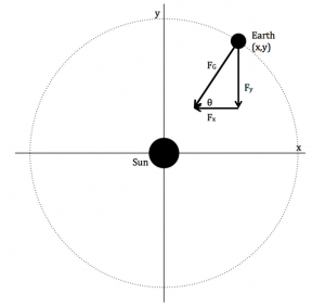
to be at the planet’s aphelion):

 v_{1} = \sqrt(\frac{G*M_{s}*(1-e)}{a*(1+e)}
 r_{1} = (1+e)*a

where a is the semi-major axis length of the planet’s orbit.

In Computational Physics, Giordano and Nakanishi find the precession of Mercury by first finding the precession rate for a much larger value of  \alpha , because it is difficult to measure the precession for a value this small (it would require computing the motion for hundreds of thousands of years). Using different values of α give different values for the precession rate, and graphing these two parameters against one another will provide the desired constant C. Once C is obtained, I can multiply this number by α to get the true precession of Mercury caused by the Sun.

Week 2: Results with Data Analysis

Once this code is working correctly, I can modify the initial conditions for the orbital motion portion of the code to represent new orbits. (Changing the parameters a, e, but maintaining the value of the perihelion as that of Mercury, so that I may compare my results to that for Mercury.)

If I have extra time I will add in other planets to the original Mercury-Sun system to observe the resulting effects on Mercury’s precession.

Week 3: Finalize project: make sure the code’s comments are informative and helpful, and review the program/results for any mistakes.

Week 4: Provide constructive criticism to other students on their projects/Prepare for project presentation.

Week 5: Give my project presentation to the class.

References:
Computational Physics by Nicholas J. Giordano and Hisao Nakanishi