Over the last two decades the cellphone has become the cornerstone of communication in our society. It has evolved to more than just a phone on the go, to become virtually a computer that fits in your pocket. The most modern cellphones on the market can not only send your voice across the country in seconds, but also send messages, e-mails, pictures, videos, stream data from the Internet, stream live TV, and even function as a wireless modem to connect other appliances to the Internet. In essence the cellphone has become the quintessential human-digital link. There are those however that worry that there might be some correlation to the radiation exuded by cellphones, and a number of health issues (e.g. brain electrical activity, cognitive function, sleep, heart rate and blood pressure). So far no correlation between the two has been found.
When searching for a correlation between cellphones and health concerns one must take into consideration the cellphone’s radiofrequency. As an apparatus, cell phones are low-powered radiofrequency transmitters, which is to say that they do emit radiofrequency but at very low ranges. Over the last two decades many organizations, including the World Health Organization (WHO) specifically The International Agency for Research on Cancer (IARC) a subdivision of WHO, the Federal Drug Administration (FDA), and the Federal Communications Commission (FCC), have run a large number of studies to ensure the safety of cellphones, and make sure that they do not have adverse effects on their users. WHO officials assure the public that “ research does not suggest any consistent evidence of adverse health effects from exposure to radiofrequency… [and that] research has not been able to provide support for a causal relationship between exposure to electromagnetic fields and self-reported symptoms” (WHO: Electromagnetic Fields and Public Health). Thus making the continual usage of cellphones safe, despite the popular notion that cellphone radiation can cause cancer or even “microwave to brain” as some radicals proclaim. Another popular argument is that cellphones have only become so widespread in the last two decades, thus the long-term effects have not been properly examined; WHO purports, however, that “results of animal studies consistently show no increased cancer risk for long-term” (WHO: Electromagnetic Fields and Public Health).
Like any other product on the market in America, cellphones have safety regulations set forth by entities like the FDA and the FCC. In conjunction, these two agencies have derived a unit called the Specific Absorption Rate (SAR), which is a measure of radio frequency energy absorbed by the body when using a mobile phone. The FCC limit on the amount of radiofrequency that cellphones can emit has been set at 1.6 watts per kg of human tissue. According the FCC website, it (FCC) “regulates the phone manufacturing industry to ensure that all cell phones emit radiation below a level that experts agree could cause health issues.” So disregard the popular notion that cellphones cause brain tumors, and keep texting away and if you are concerned about radiation from your phone please visit the FCC website: http://www.fcc.gov/guides/specific-absorption-rate-sar-cell-phones-what-it-means-you
As for our data, the average radiofrequency (RF) radiation released from smart phones during an outgoing text was 3.01V/m and for outgoing calls 3.21V/m. The average RF radiation released from non-smart phones during an outgoing text was 3.68V/m and for outgoing calls 3.59V/m. Non-smart phones show a slightly larger amount of average radiation for both texts (0.67V/m difference) and calls (0.38V/m difference). This finding was unexpected; we expected to find smart phones emitting more radiation due to their Internet connectivity and larger data bandwidth allocations. Only AT&T and Verizon had enough data to compare average radiation levels across providers. Verizon had a higher average radiation for outgoing texts, 2.67V/m to AT&T’s 2.25V/m, a difference of 0.42V/m. However, AT&T had a higher average radiation level for outgoing calls, 3.09V/m compared to Verizon’s 2.27V/m, a difference of 0.82V/m. More data would need to be collected to be more certain that these differences hold in general.
Sources of error or uncertainty in the data include changes in radiation due to the college’s Wi-Fi, and whether smart phones were Jailbroken or not. The only outlier, an iPhone 3GS with T-Mobile which had 22V/m for an outgoing text and 23.4V/m for an outgoing call, was the only phone in the data set known to be Jailbroken. Other sources of uncertainty include the orientation of the RF meter to the phone and its antenna, the proximity of other phones in crowded areas, and whether the reading was taken inside or outside.
BIBLIOGRAPHY:
Consumer Report. “How Risky Is Cell Phone Radiation?” Business Solutions & Software for Legal, Education and Government | LexisNexis. Consumers Union of U.S., Inc., Jan. 2011. Web. 30 Nov. 2011. <http://www.lexisnexis.com/hottopics/lnacademic/?shr=t>.
FCC. “Specific Absorption Rate (SAR) For Cell Phones: What It Means For You | FCC.gov.” Home | FCC.gov. Web. 30 Nov. 2011. <http://www.fcc.gov/guides/specific-absorption-rate-sar-cell-phones-what-it-means-you>.
WHO. “Electromagnetic Fields and Public Health.” World Health Organization. WHO Media Centre, May 2006. Web. 30 Nov. 2011. <http://www.who.int/mediacentre/factsheets/fs304/en/index.html>.
Our experimental data was inconsistent, which illustrates some of the problems with using lasers as a weapon. We ran two different tests with our laser in order to determine the amount of power that would be needed to realistically weaponize a laser. In the first test, we held a piece of paper in front of the laser and varied the power to record how long it would take the laser to set the paper on fire. The laser we is a green Verdi laser (wavelength = 532 nm) with a maximum power of 5 W.
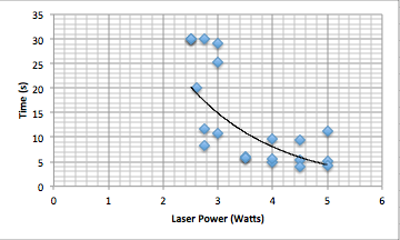
The first test we ran was the paper test. The results are presented graphically below:
As we can see, the amount of time it took the laser to burn the paper generally hovered around five seconds, with a high of 11.8 seconds. The top group represents the tests that failed to burn the paper after 30 seconds. In this experiment, we found that the minimum power needed to burn a piece of paper was 2.75 W.
The balloon data was less consistent than the paper data. We did discover that the color of the balloons had an impact on the amount of time it would take the laser to pop a balloon – pink balloons (which are much further from green on the electromagnetic spectrum then green or yellow) popped much faster and at significantly less power then either green or yellow balloons. For the pink balloons, we were able to pop a balloon instantly at only 2 W and puncture (but not pop) a balloon at 1 W. We were able to pop one green balloon at 2.5 W, but could not replicate this result when we attempted it a second time. We were able to pop both green and pink balloons at 3 W. This data tells us that the color of the target object does play a significant role in determining how much power and how long is necessary to burn or puncture a target.
The reason behind this difference is color absorption. Colors with shorter wavelengths (such as blue) reflect more light at shorter wavelengths and absorb more light at longer wavelengths. On the other hand, colors with longer wavelengths (such as red) do the opposite – reflecting more light at longer wavelengths and absorbing more light at shorter wavelengths. Since our laser was green (a shorter wavelength color), balloons that were also colors that have shorter wavelengths, such as the green and yellow balloons, should take more power and more time to pop than balloons with colors that have longer wavelengths, such as pink.
Military Applications
We saw in the lab that even at a low power of 2.75W, a laser can burn a hole through a piece of paper, or at 2W, pop a pink balloon. But how close are we to actually utilizing lasers as combat weapons? Not too far. Our research is still years away from achieving the ray guns, blasters, and light sabers that we see so much of in science fiction. Current laser weapons work by using light to excite an atom to shift its outermost electrons from one state to the next. The electrons then get ionized and torn from the atom, which leaves behind a host of positive charges. These positive charges repel and explode, and this explosion produces a wave of radiation. There are three types of lasers: gas, liquid, and solid-state. While all work in generally the same way, only gas and solid-state lasers have been utilized as weapons.
Chemical lasers, a type of gas laser, use chemical reactions to create energy. In February 2009, installed on a Boeing jet, the megawatt-class Airborne Laser (ABL) was able to shoot down long-range ballistic missiles, which could eventually progress to shooting down enemy attacks and aircrafts.The ABL is a 1.3 pm chemical oxygen-iodine laser (COIL). COILs produce a single wavelength radiation, which allows for a very well focused beam. When fired, it produces enough energy in a five-second burst to power a typical household for more than an hour.But such power comes at a price. Not just the ABL, but all chemical lasers built for the military have been bulky and logistically complex, and the cooling required to keep them running also makes them heavy. As seen in the picture, only the largest of aircrafts would be able to carry such a weapon.
Photo by Edwards Air Force Base
The need for a more efficient device prompted the government to invest money in solid-state lasers; they typically use crystal or glass as lasing media. Solid-state lasers are electrically powered, which makes them smaller and more attractive for combat, but they have only just been able to reach enough power to make them weapon-grade lasers.In the case of firearms, lasers have only been used as a tool to guide the targeting of other weapons. A laser sight for example, beams a small, visible-light laser onto a target to help aim a gun, but does no direct damage. They are now commercially available as an attachment to firearms. Other laser firearms include non-lethal laser weapons. These are typically used to disorient an opponent. The Personnel Halting and Simulation Response (or PHaSR) is a non-lethal laser weapon developed by the Air Force. It temporarily impairs aggressors by illuminating, or dazzling them, removing their ability to see the source of the laser, and is the first man-portable, non-lethal deterrent. Future uses include protecting troops and crowd control. Additional research has gone into making laser weapons that cause blindness, but the ethical considerations raised by permanently handicapping someone caused the United Nations to issue the Protocol on Blinding Laser Weapons in 1995 that forbids laser weapons whose sole purpose is to cause permanent blindness. As such, taken as a whole, the technology on building handheld laser weapons has lagged; we will not be seeing any ray guns or blasters anytime soon.
Photo by U.S. Air Force
We are making headway in solid-state lasers on a larger scale however. In 2009, engineers at Northrop Grumman Corporation were able to develop and test an electric laser that emitted 100 kW continuously for five minutes, and in April of this year, a 15 kW laser mounted on a cruiser ship was able to blast a weaving boat from the Pacific Ocean. The boat first caught fire, and then burst into flames. It is the first test at sea of such a gun and a major milestone in outfitting future Naval fleets with laser weapons. The Navy hopes to get the energy up to 100 kW and eventually take down incoming missiles.
In conclusion, existing laser weapons look promising, but they are still a long way off from reaching the ones portrayed in science fiction. Gas lasers have the potential to produce a great amount of power, but their bulk makes them inefficient to actually use in the battlefield. Solid-state lasers also have potential, but still lack the necessary power needed to create a true weapon-grade laser. But perhaps in a few years, we will finally be closer to making a little piece of fiction real.
Portrayals in Popular Culture
The Star Wars films provide us with many classic examples of laser use in science fiction. One of the most famous laser weapons in Star Wars is the Death Star – a massive space station that also functions as a high-powered laser. As shown in the clip below, the Death Star’s capabilities are quite devastating as it can destroy an entire planet. But could scientists ever develop lasers to be this powerful?
It is possible to scale our data in order to predict just how much power would be needed to achieve such a feat. We can estimate that the wavelength of this laser pulse was around 550 nm, due to the fact that the Death Star’s laser was green. Thus we can calculate the energy per photon in the Death Star’s pulse:
Energy per Photon = h*f
F = c/lambda
Lambda = 550 * 10^-9 m
C = 3*10^8
F = 5.45 * 10^14
h = 6.63*10^-34
Energy per photon = 6.63*10^-34 * 5.45*10^14 = 3.6 * 10^-19 joules per photon
In order to isolate the rate at which the Death Star emits photons, we can divide the estimated power of the Death Star (watts) by the above value.But in order to do this, we should first predict the energy that a laser would need to produce in order to explode a planet of this size/material.
The density of the earth is 5.5 grams per cubic centimeter.
The density of the paper we used for laser testing, on the other hand, has a density of .72 grams per cubic centimeter.
The ratio of the densities between these two materials is 5.5/.72 = 7.64
This ratio can be used to scale the wattage we used for paper to the wattage necessary for a planet like Alderaan.
Obviously, the destruction of Alderaan was nearly instantaneous, so we can assume a higher power is necessary for the instantaneous burning of paper. A regression analysis of our data will help us predict this new value for the instantaneous burning of paper.
Regression equation à Y = 97.251e^-.608x
Y = 97.251e^-.608(0) = 97.25 watts.
The thickness of standard paper is .103 mm. The thickness of Alderaan, of course, is much larger than this. Let us say that Alderaan has a radius similar to Earth’s: 6378.1 kilometers. We can use this radius value as the measurement of Alderaan’s “thickness.” We use it as a thickness value because we predict that a laser would only need to bore halfway through a planet in order to destroy it. There are two reasons for this. First of all, as we mentioned in the earlier in our post, the ionized particles that are shot from a laser repel each other, resulting in an “explosion” effect. The second reason has to do with a process called spallation. Spallation occurs when a high-powered laser cuts through a rock, heating up the moisture contained within that rock. Vapor within the subsurface of the rock begins to explode outwards, which results in a high degree of stress on the overall system. Alderaan is one big rock, most likely trapping a large amount of moisture within its subsurface. Therefore the laser would only need to travel far enough to result in a heating of the inner layer of Alderaan, resulting in an explosion.
Thus for our purposes, we will use the planet’s radius as its “thickness” value. The ratio of the planet’s thickness to the paper’s thickness is…
(6378.1*10^3)/(*10^-3) = 6.2*10^10
Using these ratios, we can use the effective power of our lab laser in order to predict the effective power of the Death Star.
Death Star Power = Lab Laser Power (for instantaneous burning of paper) * Thickness Ratio * Density Ratio
Death Star Power = 97.25 * (6.2 * 10^10) * 7.64 = 4.6*10^13 watts
This is the minimum number of watts the Death Star would need in order to generate a laser that could destroy Alderaan. Given the Power, and the Energy per photon of the Death Star’s laser, we can also find the rate at which the Death Star emits photons.
Power = Rate of photon emission * energy per photon
4.6*10^13/3.6*10^-19 = 1.28 * 10^32 photons per second
Given today’s standards of technology, these are incredibly large numbers for power output and photon emission rate. However, new developments in laser technology suggest that it could be possible for a laser to be built with these power specifications. For example, scientists are currently building an unprecedented laser that can produce 200 * 10^15 watts of power. This laser is unlikely to be militarized, however; researchers will use it to investigate the nature of matter and antimatter particles in space. Still, it seems that the writers of Star Wars created the Death Star with relatively good scientific underpinnings. Interestingly, if you closely watch the Death Star clip, several of its lasers appear to “join” together before creating a unified, larger laser. This appears to violate very basic properties of light – light beams would not “join together” upon intersection. Rather, they would simply pass right by one another and continue heading in a straight direction. However, the aforementioned “super laser” under construction does combine multiple lasers into one “focal point” that results in a single, incredibly powerful beam.
Thus, Star Wars appears to have a decent amount of science behind its fictional technology.
Blaylock, Eva D. (November 2005). New technology ‘dazzles’ aggressors.” U.S. Air Force. http://www.af.mil/news/story.asp?storyID=123012699
Erwin, Sandra. (December 2002). Tactical laser weapons still many years away. National Defense 87.589 32-33. http://search.proquest.com/pqrl/docview/213398105/fulltext?accountid=14824
Hecht, Jeff. (April 2010). A new generation of laser weapons is born. Laser Focus World 46.4. http://search.proquest.com/docview/228075969
ICRC. (October 1995) Protocol on Blinding Laser Weapons (Protocol IV to the 1980 Convention). International Humanitarian Law – Treaties & Documents. http://www.icrc.org/ihl.nsf/0/49de65e1b0a201a7c125641f002d57af?OpenDocument
Kaplan, Jeremy A. (April 2011). Navy Shows Off Powerful New Laser Weapon. Fox News. http://www.foxnews.com/scitech/2011/04/08/navy-showboats-destructive-new-laser-gun/?test=faces
Tech. Sgt Grill, Eric M. (January 2007). Airborne Laser returns for more testing. Air Force Material Command. http://www.afmc.af.mil/news/story.asp?id=123038913
Photos:
Edwards Air Force Base. Accessed 29 November 2011. http://www.edwards.af.mil/news/story.asp?id=123046780
U.S. Air Force. Accessed 29 November 2011. http://www.af.mil/news/story.asp?storyID=123012699
Tomorrow, we will present the following data on computer use at Vassar:
Department
# Computers
Note(s)
Anthropology
8
Art
19
Biology
25
Chemistry
23
Chinese/Japanese
8
Computer Science
9
Dance
10
Drama
12
Earth Science/Geography
9
Economics
13
Education
9
English
31
Film
10
Franch and Francophone
8
**
German
4
**
Hispanic
8
**
History
17
Italian
7
**
Mathematics
9
Music
40
*
Philosophy
9
Physical Education
27
*
Political Science
13
Psychology
21
Religion
9
Russian
4
**
Sociology
10
We will present our findings by making categorizes of computer usage based on academic field (i.e. Science, humanities, etc…)
We will address the issues we faced regarding getting more data regarding energy usage.
Finally, we will present what we seek to calculate, using a watts up pro, and the map we will create using those results.
We will include the following results:
To Note:
-This data does not include public (for class use) and personal (for professors’ research) labs in any of the departments, particularly the biology, chemistry, physics and astronomy, computer science, mathematics, and psychology departments. Without access to a number of the labs, it is impossible to estimate how many computers are utilized without being inaccurate and biased to some extent. Therefore, we are only examining the energy used in each academic department’s office. Thus, energy use will correlate with size of department.
-According to the office of computer information services (CIS), each faculty and staff member in a department should have one computer (although some do bring in their own laptops in addition to their office desktop, according to CIS). Therefore, we calculated the number of computers in each academic department through estimating that the number of faculty and staff in a given department equals the number of computers in that department. Because of this, there is certainly a great amount of room for error, as some faculty and staff could use more than one computer (or possibly not use a computer at all, although that is extremely unlikely), some professors work in multiple departments and only utilize one office, and some offices have extra computers for student use. Furthermore, according to CIS the models of the computers vary, but we are unable to take into account which computers require more energy than others, thus we treated all computers equally in terms of energy expenditure. So while our results may not be 100% accurate, we should be able to give a rough estimate of how much energy each department office utilizes.
-We only calculated academic departments; we did not include any academic programs (e.g. Africana Studies, Cognitive Science, Urban Studies etc.). We followed the Vassar College catalogue’s categorization of departments and programs.
-Computers of professors who are on sabbatical were not included in this data, as they are most likely not utilizing their office computers this term.
KEY:
*One very important note for the music and physical education departments: while their numbers seem to be huge, this is misleading. For the music department, faculty and staff include visiting artists and instructors (such as voice teachers and accompanists), and these individuals either share computers or do not have one at all. For the physical education department, faculty and staff include coaches and assistant coaches, who may share computers. Perhaps we shouldn’t include them in this study?
**These language departments share administrative assistants, but just in case one computer has been added to each department.
We set out to measure the strength of the wireless Internet signal across campus and create a heat map detailing the relative differences we found. Our hypothesis was that the Internet signal would be relatively uniform across most of campus and in the dorms/academic buildings, increasing when we got particularly close to an airport. We expected lower readings at the edges of campus and around Sunset Lake, where we already knew that the wireless Internet does not.
Technology and Procedure
We used an RF meter to measure electric field strength in mV/meter. We hoped to single out a wireless Internet signal, but the technology was unable to accomplish this. We walked around campus with the RF meter, measuring electric field strength in various predetermined locations.
Findings
Electric field strength outdoors was quite consistent, ranging from 4-7 mV/meter. There was no noticeable difference in electric field strength between central campus and campus’ outer edges/Sunset Lake. Inside the buildings electric field strength generally ranged from 100-300 mV/meter. Of the dorms we found that Jewett had the weakest electric field strength, of around 100 mV/meter, while Joss had the greatest, of around 350 mV/meter. We found the greatest electric field strength of all in the fitness room of Walker, it being about 500 mV/meter. Here is a google map with all of our findings: <http://maps.google.com/maps/ms?ll=41.688617,-73.894944&spn=0.008156,0.01369&t=m&z=16&vpsrc=6&msa=0&msid=216952304120227955446.0004b2fc32482f27e766d>
Complications with the project
We encountered a few problems throughout our project. First, the RF meter was unable to single out the wireless internet signal, so any other electronics in the area affected our data. Second, the readings we took outside were all very consistent, even when we expected a difference in readings. For example, we know that the internet signal does not reach the area around Sunset Lake, but we got the same reading in that area as we got in the quad (where we know the internet signal does reach). This could be due to other signals (cell phone towers, radio, etc.) giving a consistent signal everywhere outside and drowning out the changes in wireless internet signals.
Conclusions
While we did not get accurate data for the strength of the wireless internet signal, we were able to compare the strength of electric fields in buildings around campus. The highest reading we found was in the Walker fitness center, where it reached 500 mV/meter. This could be due to all the electric equipment in the gym, such as treadmills and TVs. The lowest readings were found mostly in dorms (Joss, Noyes, Jewett, etc.) and were all around 100-200 mV/meter. All of these readings should be taken with a grain of salt, however, as they were very dependent on proximity to electric devices.
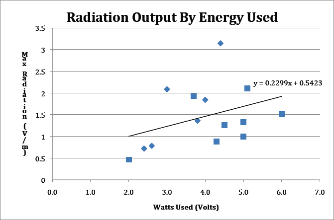
Our group conducted research to determine if there is any correlation between how much energy a cell phone uses and how much radiation it emits. We recorded the energy used by measuring the amount of power necessary to run the phone while it made a one minute phone call. The power ran from the wall through the Watts Up Pro to the phone charger, and finally to the phone. This gave us the number of watts used, displayed in the table below. We measured the radiation emitted using the RF meter, which gave us radiation in volts per meter.
Watts Used
Max Radiation (V/m)
Phone Type
Smart Phone?
2.0
0.465
Droid Incredible 2
Yes
2.4
0.720
Verizon LG
No
2.6
0.783
Verizon flip phone
No
3.0
2.087
Verizon LG
No
3.7
1.929
Droid 1
Yes
3.8
1.361
Verizon LG
No
4.0
1.843
Verizon LG
No
4.3
0.884
Droid 2
Yes
4.4
3.145
Samsung
No
4.5
1.262
Droid X
Yes
5.0
1.333
Droid 2
Yes
5.0
0.992
iPhone 4
Yes
5.1
2.111
iPhone 4
Yes
6.0
1.507
iPhone 4S
Yes
Our data shows that phones that use fewer watts do, in fact, emit less radiation. The graph displays that there is some correlation. However, to identify this trend conclusively more research is required. The data suggests that smart phones use, on average, more energy than phones without those capabilities, known as feature phones. Six of the top seven power-using phones we tested were smart phones, while the majority of the remainder were feature phones. While the smart phones may use more power, they don’t appear to emit more radiation. It is possible that phone makers work harder to reduce the amount of radiation emitted by their more expensive models. A potential source of error in our experiment could be that we tested phones of different service providers. Phones with bad service in the area we tested them (the Retreat) probably had to work harder (and use more energy) to get service during the call. To find a true correlation, if there is one at all, we would need to take more data and take phone providers into account. Our data suggests that there may be a correlation, which certainly warrants more investigation.
Our experiment returned different results than we expected. Initially we were expecting the tests we performed (nitrate and copper tests) to give us sufficient evidence to classify our two water sources—the Hudson River and Sunset Lake—as non-potable. However, as we discovered, the nitrate and copper levels are sufficiently low to be below the EPA’s cut-off for potability. We were disappointed by this outcome, as we had hoped to prove, beyond a shadow of a doubt, that the water sources were dangerous to drink. In the future, given more time, we would like to have been able to perform tests to determine bacteria levels in the water, such as E. coli or other coli-form bacteria, and the levels of other organisms, such as Giardia. We would expect the levels of these bacteria and organisms to be too high to allow for safe drinking. Perhaps the spectroscopy readings suggest the presence of things other than simply water molecules, as the Hudson River and Sunset Lake had higher absorbance in the violet range of the spectrum than regular drinking water.
This experiment, while perhaps unsuccessful in terms of what we had hoped to discover, is a good example of why one or two negative tests do not necessarily account for all possible contaminants.
In conclusion, despite the negative results from our tests, we would still suggest that you choose not to drink from the Hudson or Sunset Lake.
For our data collection we used the RF meter to measure the strength of electric fields around campus, ultimately to judge the relative strengths of wireless signals across the school. The values are all in mV/m. We will have more data points in the coming week, covering the rest of campus
For our data, we tested the wattages and times it would take a green laser to burn paper and to pop various colors of balloon. For our paper tests, we recorded the laser’s power and how long it took to burn the paper. For the balloon tests, we recorded power, the balloon’s color, and how long it took to pop the balloon.
We tested twenty individuals for our study. Each individual listened to three music clips. The right speaker played a volume adjusted remastered recording while the left side played a volume adjusted original track. Each participant was asked to rate the sound quality for each side of each recording on a scale of 1 to 10 based on preference and sound quality adding any adjectives to describe the differences between them as needed.Furthermore, since some of the clipping in the tracks occurs at very high sound frequencies, a hearing range test was also given. To compensate for individual sound quality scale differences, the differences between the two sides was also averaged, not just the average rating of each side’s sound clip.
Wild World
Voodoo Child (Slight Return)
Man In The Box
Subject Number:
Hearing Range:
Left:
Right:
Left:
Right:
Left:
Right:
1
20 Hz – 19 KHz
5
6 (clearer, louder)
6
4 (grainy vocals)
8
8 (louder)
2
20 Hz – 18 KHz
4
6 (clearer)
6 (clearer)
4 (fuzzy)
6
6 (louder)
3
20 Hz – 19 KHz
3 (fuller)
2
3
2
4
4
4
20 Hz – 20 KHz
7 (clearer, deeper)
6
8.25 (more layers, better tone)
7.25
7.75
7.5 (less tonal depth)
5
20Hz – 17 KHz
8 (clearer, louder)
7
7 (clearer)
6.5 (grainy lower sound)
7
6.5 (louder)
6
20 Hz – 18 KHz
6 (warbly)
9
8 (crisp)
5 (fuller, deeper)
5
7
7
20 Hz – 16 KHz
7 (more sound)
6
8 (more percussion)
8
7
7 (louder)
8
20 Hz – 18 KHz
5 (muddier)
7 (cleaner)
6 (instruments easier to pick out)
5 (more mids)
6 (more high end)
7 (higher sound quality)
9
20 Hz – 18 KHz
6.5 (flatter)
5 (fuller)
6.25 (punchy drums)
4.75 (muted drums)
5.75
7 (punchy drums, fuller singing)
10
20 Hz – 17 KHz
6 (more subdued)
7 (fuller)
7 (heavier drumming)
5 (tinnier)
7
8 (louder)
11
20 Hz – 20 KHz
6 (softer)
8 (more crisp)
6 (heavier)
4 (muted)
7
7 (louder, fuller)
12
20 Hz – 18 KHz
8 (more delicate)
5 (too loud)
8 (more powerful)
6 (distant)
7
6 (louder)
13
20 Hz – 19 KHz
6
8
9 (more crisp)
7 (fuzzy)
8
6 (louder)
14
20 Hz – 16 KHz
7
6 (louder, fuller)
7 (richer)
6 (less clear)
6
7
15
20 Hz – 17 KHz
5 (too soft)
7 (fuller)
7 (clearer)
4
6
8 (louder)
16
20 Hz – 20 KHz
5 (clearer)
4
6
3 (very grainy)
6 (deeper)
5 (louder)
17
20 Hz – 18 KHz
7
6 (stronger)
8 (more dynamic)
6 (flatter)
6
6
18
20 Hz – 19 KHz
6 (flatter)
8
9
7
7
8 (louder)
19
20 Hz – 16 KHz
5
6 (clearer)
7 (clearer)
5
5
6 (louder)
20
20 Hz – 19 KHz
8 (fuller bass)
6.5
7 (muffled)
8 (clearer)
7 (muffled)
8 (clearer)
Average
20Hz-18.1KHz
6.025
6.275
6.925
5.375
6.425
6.75
The average preference for Wild World was 0.1 in favor of the remaster. The Average preference for Voodoo Child (Slight Return) was 1.1 in favor of the original recording. And the average preference for Man in the Box was 0.25 in favor of the remaster.
Thus far, we have been notified by CIS of each department’s computer usage.
We are waiting for Buildings and Grounds, and the Department Chairs to notify us of #rooms and special equipment per department. We may have to alter our methodology based on what the various departments provide us with.
However, it is important we have computer information, because we can assume they are all the same type of computer, and that will help us when we calculate results, and conclude on our findings.
Department
# Computers
Note(s)
Anthropology
8
Art
19
Biology
25
Chemistry
23
Chinese/Japanese
8
Computer Science
9
Dance
10
Drama
12
Earth Science/Geography
9
Economics
13
Education
9
English
31
Film
10
Franch and Francophone
8
**
German
4
**
Hispanic
8
**
History
17
Italian
7
**
Mathematics
9
Music
40
*
Philosophy
9
Physical Education
27
*
Political Science
13
Psychology
21
Religion
9
Russian
4
**
Sociology
10
To Note:
-This data does not include public (for class use) and personal (for professors’ research) labs in any of the departments, particularly the biology, chemistry, physics and astronomy, computer science, mathematics, and psychology departments. Without access to a number of the labs, it is impossible to estimate how many computers are utilized without being inaccurate and biased to some extent. Therefore, we are only examining the energy used in each academic department’s office. Thus, energy use will correlate with size of department.
-According to the office of computer information services (CIS), each faculty and staff member in a department should have one computer (although some do bring in their own laptops in addition to their office desktop, according to CIS). Therefore, we calculated the number of computers in each academic department through estimating that the number of faculty and staff in a given department equals the number of computers in that department. Because of this, there is certainly a great amount of room for error, as some faculty and staff could use more than one computer (or possibly not use a computer at all, although that is extremely unlikely), some professors work in multiple departments and only utilize one office, and some offices have extra computers for student use. Furthermore, according to CIS the models of the computers vary, but we are unable to take into account which computers require more energy than others, thus we treated all computers equally in terms of energy expenditure. So while our results may not be 100% accurate, we should be able to give a rough estimate of how much energy each department office utilizes.
-We only calculated academic departments; we did not include any academic programs (e.g. Africana Studies, Cognitive Science, Urban Studies etc.). We followed the Vassar College catalogue’s categorization of departments and programs.
-Computers of professors who are on sabbatical were not included in this data, as they are most likely not utilizing their office computers this term.
KEY:
*One very important note for the music and physical education departments: while their numbers seem to be huge, this is misleading. For the music department, faculty and staff include visiting artists and instructors (such as voice teachers and accompanists), and these individuals either share computers or do not have one at all. For the physical education department, faculty and staff include coaches and assistant coaches, who may share computers. Perhaps we shouldn’t include them in this study?
**These language departments share administrative assistants, but just in case one computer has been added to each department.