Category Archives: Mix and Measure Colors Workshop

Science Matters at Dutchess Community College: Mix and Measure Colors Workshop held by Prof. Magnes from Vassar College.

Orbital Motion Simulation – Frye and Gittins


We plan on modeling objects in orbital motion, namely the sun and earth, the earth and moon, the three together, and finally an orbit of two large-massed bodies, such as the sun and another star.

The programming steps we need to take are straightforward in theory. We have already settled on using the Euler-Cromer method on MatLab to simulate the motion. We have access and prior knowledge of Newton’s laws and Kepler’s laws of motion, as shown below.  The potentially difficult part will be writing a program that will be able to track the motion of several bodies simultaneously, with the capability of visualization, such as a moving graphic.


(1)   \begin{equation*} \ F_{G}=\frac{GM_{S}M_{E}}{r^{^{2}}} \end{equation*}


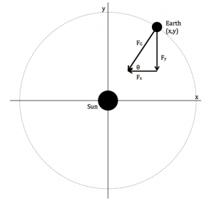
where Ms is the mass of the sun and Me is the mass of the earth.


Kepler’s Laws:

  • All planets move in elliptical orbits with the Sun at one focus.
  • The line joining a planet to the Sun sweeps out equal areas in equal times.
  • If T is the period and a the semimajor axis of the orbit, then T^2/a^3

(2)   \begin{equation*} \frac {d^{2}x}{dt^{2}} = \frac {F_{Gx}}{M_{E}} \end{equation*}

(3)   \begin{equation*} \frac {d^{2}y}{dt^{2}} = \frac {F_{Gy}}{M_{E}} \end{equation*}


from which we can derive the equation:

(4)   \begin{equation*} \ F_{Gx}=-\frac{GM_{S}M_{E}}{r^{2}}\cos{\theta}=-\frac{GM_{S}M_{E}x}{r^{3}} \end{equation*}

for the x-direction. A similar equation can be found for the y-direction. For the equations of motion that will be put into the Euler-Cromer program, we will use equations similar to those derived in Giordano.


(5)   \begin{equation*} \ v_{x,i+1}=v_{x,i}- \frac{4\pi^{2}x_{i}}{r_{i}^{3}}\Delta{t} \end{equation*}

(6)   \begin{equation*} \ x_{i+1}=x_{i}+v_{x,i+1}\Delta{t} \end{equation*}

(7)   \begin{equation*} \ v_{y,i+1}=v_{y,i}- \frac{4\pi^{2}y_{i}}{r_{i}^{3}}\Delta{t} \end{equation*}

(8)   \begin{equation*} \ y_{i+1}=y_{i}+v_{y,i+1}\Delta{t} \end{equation*}


For preliminary data, we hope to have a primitive program that has the capability of simulating a simple Earth-Sun orbit, assuming that the Sun is so massive (compared to Earth) that it does not move. We hope to have an appropriate visualisation, a moving plot, to apply to the data. At this time we will need to heavily research the physics of the situation, including providing details of what is physically incorrect about our simulation and the amount of error these details create. The defense of this simulation, including pros and cons of the Euler-Cromer method in this case, will be in the preliminary data.

The second goal is to make the system more complicated, either adding the moon or another planet to the existing system. As in the first set of data, we will need to analyze it for flaws. We anticipate this to be the most difficult programming challenge, as there are three systems moving simultaneously, and also the most complex error analysis.

Screen Shot 2015-04-01 at 12.10.11 AM

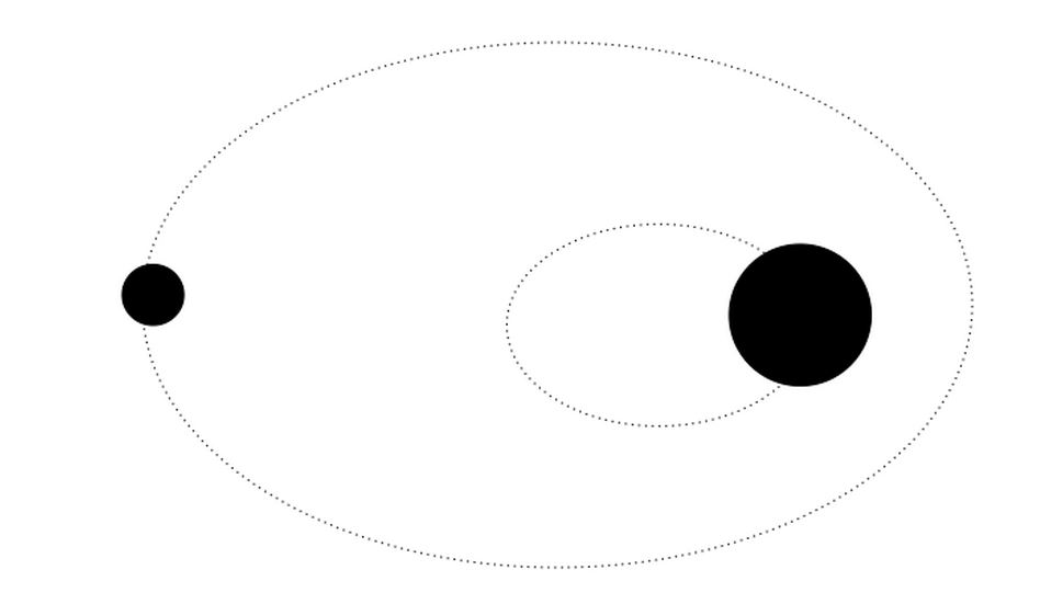
Finally, we plan to model a system in which each mass is in motion, for example, two large suns or a star and a large planet.  At this point, we will be fairly comfortable with the Euler-Cromer method applied to this system. Here, we will truly analyze the flaws with the method and compare and contrast these flaws, and its strengths, with other methods we have learned in class. This will also provide insight into our previous simulations and their errors, as the sun is not un-moving as we assume previously.

two massiv

We hope the final program will appear similar to the ones shown in Giordano and the exploration of orbits done by Moler.


Timeline:

Week 1: Research more equations and pseudo codes that relate to our simulation.

Week 2: Write a primitive program to simulate the earth and the sun orbit. Calculate error.

Week 3: Finish Earth-Sun simulation. Begin writing program for Moon-Earth-Sun by working with program from Week 2. Begin writing primitive program for two massive planets or stars.

Week 4: Finish program for two massive planets or stars. Calculate error. Troubleshoot Moon-Earth-Sun program.

Week 5: Finish all programs and prepare for presentations.


Resources

  1. Giordano. Computational Physics, 2006.
  2. Moler, Cleve. “Orbits,” MathWorks Inc, 2011.
Share

Project Plan Monte Carlo Simulation Financial Applications

The first objective of our project is to use MatLab to provide simple examples of how the Monte Carlo method can be used. To do this I will create a simple program that shows the distribution of numbers of a six-sided die land on when randomly thrown for a specific number of iterations. To do this I will use the basic method of the Monte Carlo method provided by our textbook Computational Physics by Nicholas J. Girodano and Hisao Nakanishi. The second program I will create will demonstrate how the Monte Carlo method can be used to find the moment of inertia for an object with a range of different measurements for different parameters. Finally the third simple program I will create will be using the Monte Carlo method to find how much money someone needs to be invested into a stock or portfolio of stocks to retire at certain age. All these simple programs use the concept of normal or lognormal distribution and take advantage of MatLab’s built in random number generator. With these simulations we will discuss how central limit theory provides a basis for the Monte Carlo method being an acceptable

The second goal of our project, Elias Kim and I will both attempt to use the Monte Carlo algorithm for the Ising model on an L x L square lattice, separately. The Ising model is an integral part of physics because it helps describe how neighboring atoms and their electron magnetic spins interact with one another and have the ability to change the neighboring electrons spin. In addition the Ising model is used to explain ferromagnetic interaction but its influence has extended into the world of thermodynamics as well. Elias and I will then join together to compare our answers to make sure we got similar solutions.

The final objective of our project, Elias and I will team up and use our knowledge of the Monte Carlo method and Ising model to tackle financial problems. The Ising model can be used to exam the volatility of a stock or portfolio and the risk associated with it. In the world of finance, volatility is defined as a statistical measure of the dispersion of returns for a given security or market index, this can be simply calculated with the standard deviation of returns from that same security or market index. Many factors that previously were thought as random actually alter the volatility of an asset, which is what Elias Kim, and I intend to investigate.


Timeline:

Week of April 6th : Acquire basic knowledge of Monte Carlo simulation and relevant equations and concepts. Continue researching about the Ising Model and various financial principles.

Week of April 13th : Create the three basic Monte Carlo simulations described in the General Plan, and begin to work on the simple Ising Model described in Computational Physics.

Week of April 20th :Finish the simple Ising Model, and compare results to Elias’ findings . Continue researching the Ising Model and its applications to the financial world.

Week of April 27th: Begin working on the applying the Ising Model to a financial problem. Continue researching on the Ising Model and its applications to finance.

Week of May 4th : Finish the collaboration with Elias and get ready for project presentations.

References:

1. Monte Carlo Techniques G. Cowan (RHUL).

2. Probability Review and Overview of Monte Carlo Martin Haugh

3. http://www.excelfunctions.net/Excel-Norminv-Function.html ExcelNet

4. Ising Model in Finance Pavel Dvoˇr´ak

5. Physics and Financial Economics (1776-2014): Puzzles, Ising and Agent-Based models

D. Sornette (ETH Zurich)

6. Phase transition in an Ising economy Miloš Borovšak

7. Statistical physics of social dynamics Claudio Castellano, Santo Fortunato, Vittorio Loreto

8. Computational Physics Nicholas J. Girodano, Hisao Nakanishi

Share

Project Plan: Monte Carlo Method and its applications in Finance

Theoretical Motivation:

During the final stages of the Manhattan Project, Stanislaw Ulam and John Von Neumann developed the Monte Carlo method in order to calculate on average how long it would take for a neutron to collide with the nucleus of an atom when projected into a given substance. Named after the famous Monaco casino, Monte Carlo methods are often used to describe systems that have a set range of inputs and parameters, the specifics of which are unknown. The method inputs random or pseudo-random values into the system over and over again to see if a certain trend emerges when certain combinations of values are chosen. Often, Monte Carlo methods are used to simulate systems in physics that have many coupled degrees of freedom, such as radiation and fluid dynamics. However, many social scientists have since begun to use Monte Carlo simulations to predict the ways that certain trends develop, particularly in the world of finance and economics.

The Ising model emerged from the study of ferromagnetism, providing a way to study the interactions between adjacent atoms with discrete magnetic spin numbers. Since each spin influences its surrounding neighbors, these systems are modeled by creating a grid of cells that influence the cells around it based on a specific set of laws or equations. In the context of physics, the Ising model has since expanded from the field of ferromagnetism into thermodynamic phase transitions and other related fields. Like the Monte Carlo method, it has also been commandeered by the finance community to map the progress of interrelated variables and actors in an economic system. It does so by defining a set of actors governed by mutual economic and financial laws.

Finally, in the world of finance, volatility refers to the way that a financial instrument’s price changes over time. Many traditional models of volatility follow a deterministic approach in which the price of a financial security (any type of financial asset) has a constant volatility over time. However, these models often fail because the volatility of any given security is in reality stochastic over time and evolves due to the contributions of many factors, some of which cannot be seen directly. To account for this stochastic volatility when determining the price of financial assets, economists have often turned to Monte Carlo methods and the Ising model to predict the way interrelated, seemingly random factors evolve over time. Adam Warner and I plan to gain a preliminary understanding of the way that these methods transfer from physics to the world of finance.

Description:

I will begin my study by using MatLab to write very basic examples of both an Ising system and an independent Monte Carlo method, starting with the discussion in Giordano’s computational physics. I will then use a Monte Carlo simulation to solve a more rigorous physics problem, concerning the emission of radiation from an atom. This process is stochastic in nature, so I believe it will be a good precursor to looking at the kind of method necessary to solve a financial volatility problem. I will then attempt to model the volatility of a derivative security, a financial asset that depends on the prices of other more basic assets. Finally, if time allows, Adam and I will work together to develop an Ising model that describes an economic system.

Timeline:

Week 1 (4/6-4/12)

I will finish my research on the basic principles of the Ising Model, Monte Carlo Methods, and Volatility. I would like to have a comprehensive list of papers to reference and be ready to start working in MatLab.

Week 2 (4/13-4/19)

At this point, I will start to work on my models for the basic Monte Carlo and Ising problems. I do not think that these will be too rigorous and I hope to be able to display these in my first preliminary results report. I will need to figure out the kind of notation to use for this sort of computation.

Week 3 (4/20-4/26)

By then, I should be ready to start my model of atomic radiation. This will help me get a good grasp on how to approach a stochastic system in MatLab and should be an example of some pretty interesting physics concepts. I hope to get this into my preliminary results as well, but am less certain.

Week 4 (4/27-5/3)

Now, I will attack the meat of my project. I will use all of the concepts I have worked with up to this point to model the stochastic evolution of the volatility of derivative security.

Week 5 (5/4-5/10)

This week I should be able to finish the model described previously. If all goes according to plan, I will have time to work with Adam on characterizing how an Ising model would be able to describe the evolution of interconnected securities and the decisions made to give them prices.

Sources:
1. Computational Physics, Giordano and Nakanishi
2. Physics and Financial Economics (1776-2014): Puzzles, Ising and Agent-Based models
D. Sornette (ETH Zurich)
3. University of Virginia: Introduction to Atomic Simulations, Leonid Zhigilei
4. Probability Review and Overview of Monte Carlo, Martin Haugh
5. Monte Carlo Methods for Security Pricing, Phelim Boyle, Mark Boardie, Paul Glasserman
6. Monte Carlo simulation of the atomic master equation for spontaneous emission
R. Dum, P. Zoller, and H. Ritsch

Share

Precession of Mercurian Planets: Project Plan

Goals:

For my computational physics project I would like to investigate the relationship between the precession and the eccentricity of a planet’s orbit due to general relativity as detailed in chapter 4, section 3 of Computational Physics, by Nicholas J. Giordano and Hisao Nakanishi. The rate of precession examined in this project will only be that which is caused by the general relativistic effect of the model planet’s host star.

Week 1: Preliminary Results

As a check to make sure my code will run correctly, I will first model the precession of Mercury’s orbit as caused by the Sun. I must first write a code that will model the movement of a Mercury through it’s orbit according to Kepler’s laws. The force law predicted by General Relativity is given by:

 Fg=\frac{GM_{s}M_{m}}{r^{2}}(1+\frac{\alpha}{r^{2}})

where G is the Gravitational constant of the universe, Ms is the mass of the Sun, Mm is the mass of Mercury, and a Constant*α gives the rate of precession for the orbit. For the case of Mercury,  \alpha=1.1*10^{-8} AU^{2} .

Applying the Euler-Chromer method to the above equation to approximate the x and y velocities and positions of the planet as it travels throughout its orbit yields:

 V_{x,i+1}= V_{x,i}-(4*(\pi^{2})*x_{i})/(r_{i})^{3}+(\alpha*4*(\pi^2)*x_{i})/(r{i})^{5})*\Delta(t)
 x_{i+1} = x_{i}+(V_{x,i+1})
 V_{y,i+1}= V_{y,i}-(4*(\pi^2)*y_{i})/(r_{i})^{3}+(\alpha*4*(\pi^{2})*y_{I})/(r_{I})^{5})*\Delta(t)
 y_{i+1} = y_{i}+(V_{y,i+1})

Where the initial conditions are (assuming  r_{1} to be at the planet’s aphelion):

 v_{1} = \sqrt(\frac{G*M_{s}*(1-e)}{a*(1+e)}
 r_{1} = (1+e)*a

where a is the semi-major axis length of the planet’s orbit.

In Computational Physics, Giordano and Nakanishi find the precession of Mercury by first finding the precession rate for a much larger value of  \alpha , because it is difficult to measure the precession for a value this small (it would require computing the motion for hundreds of thousands of years). Using different values of α give different values for the precession rate, and graphing these two parameters against one another will provide the desired constant C. Once C is obtained, I can multiply this number by α to get the true precession of Mercury caused by the Sun.

Week 2: Results with Data Analysis

Once this code is working correctly, I can modify the initial conditions for the orbital motion portion of the code to represent new orbits. (Changing the parameters a, e, but maintaining the value of the perihelion as that of Mercury, so that I may compare my results to that for Mercury.)

If I have extra time I will add in other planets to the original Mercury-Sun system to observe the resulting effects on Mercury’s precession.

Week 3: Finalize project: make sure the code’s comments are informative and helpful, and review the program/results for any mistakes.

Week 4: Provide constructive criticism to other students on their projects/Prepare for project presentation.

Week 5: Give my project presentation to the class.

References:
Computational Physics by Nicholas J. Giordano and Hisao Nakanishi

Share

Drunken MATLAB Journey

Dillon Guynup

Computational Physics

I would like to explore a very important question at our college: will I make it back to campus if I am taking steps in random directions this weekend? Starting from the Town Houses, what is the probability of making it back to my room while quite inebriated? In 2 dimensions, this is nigh guaranteed but how many steps will it take? By manipulating the distance traveled, I can find a trend in the average number of steps the student takes and fit a trend line to it.

Not only can this be mapped in MATLAB, I can also insert extra variables into the program. For example, I can introduce non-random movement at random times. In the real world, this could be seen either as a moment of clarity in a drunken mind or a helpful friend pushing you in the right direction. I would like to derive the expression to calculate the number of steps to go back to campus computationally. This could be an example of random drift and could be used to see how drift affects the time it takes to go home. I can add a lot more to this project by utilizing even more variables. For example, what if the student slips? I could add another random chance of a non-random movement this way.

Share

Project Proposal Matt Dubow

For my computational project I would like to investigate two particular topics in celestial mechanics: the precession of the perihelion of Mercury and Kirkwood gaps. Astronomy is a very precise science, but nevertheless deviations from the accepted laws exist, and sometimes the exact results are poorly known; in these situations computational answers are the most useful and feasible. One such deviation from the accepted laws (here, Kepler’s laws) is the precession, or the rotation of the orientation axes of its orbit, of the planet Mercury- that is, the point at which Mercury is closest to the Sun rotates moves, most likely due to the gravitational effect from the other planets. This precession can be calculated using computational methods. A similar situation arises with the asteroids that orbit in our solar system- something, most likely the gravity of other planets, is causing a deviation from known laws, only here, the asteroids are conspicuously absent from certain orbital radii. The gaps, mostly caused by Jupiter, are referred to as Kirkwood gaps and are found at particular orbital resonances with Jupiter (i.e. 2/1, 3/1, 5/2 resonances). The same process occurs with the rings around a planet such as Saturn- for some orbital radii there is no such ring. The occurrence of such gaps, in orbital location and at resonance point, can be found via computational methods.

Share

Computational Physics Project Proposal – Vibrations, Waves, and the Physics of Musical Instruments

Computational Physics Project Proposal

Greg Cristina

Teddy Stanescu

Chapter of interest: Ch 11 – Vibrations, Waves, and the Physics of Musical Instruments. For this project, We want to explore different aspects of vibrations and waves as they occur in musical instruments. In general, we would like to explore everything in this chapter. This can involve modeling string displacement and decay through plucked and struck strings as well as analyzing the frequencies produced. We can also compare this data calculated in MatLab to a real life setting, recording a string being plucked or struck, then using measurements to model the same scenario in MatLab, then compared calculated vs. actual results. Also we would like to explore the overtones of the sounds generated and see if it correlates to the frequencies found using a Fourier Transformation on the recorded frequencies. If we have enough time, we would also like to repeat these experimental steps with a drum, exploring the way waves travel on a circular plane with locked or heavily damped edges (the rim of the drum). The drum can be struck in the center of the drumhead or the center and the rim at the same time, producing two different sounds and wave patterns.

Share

Random Weekend Motion

Dillon Guynup

I would like to explore a very important question at our college: will I make it back to campus if I am taking steps in random directions this weekend? Starting from the Town Houses, what is the probability of making it back to my room while quite inebriated? In 2 dimensions, this is nigh guaranteed but how many steps will it take? By manipulating the distance traveled, I can find a trend in the average number of steps the student takes and fit a trend line to it. This should allow me to derive the expression for random movement.

Not only can this be mapped in MATLAB, I can also insert extra variables into the program. For example, I can introduce non-random movement at random times. In the real world, this could be seen either as a moment of clarity in a drunken mind or a helpful friend pushing you in the right direction. I would like to derive the expression to calculate the number of steps to go back to campus computationally. This could be an example of random drift and could be used to see how drift affects the time it takes to go home. I can add a lot more to this project by utilizing even more variables. For example, what if the student slips? I could add another random chance of a non-random movement this way. That’s about it, folks.

Share

John Loree Project Proposal

I am currently working on a senior thesis in Physics. As part of this project, I intend to harvest nerve spike train signals using either an EMG apparatus or a fine-needle electrode direct to the nerves in interest. These signals tend to be obscured heavily by noise, and as such are difficult to use experimentally. For this project, I intend to use a Fourier Transform or other computational methods to separate out EMG signals from background noise, and extract the relevant parameters from those nerve signals (duty cycle frequency, peak cycle stress) that can be used to help control a robotic agent elsewhere in my project.

Share