The primary goal of this week was to further our understanding of the Monte Carlo method works. To do this we researched basic modes of how the Monte Carlo method operates. The Monte Carlo method relies on the repeated random sampling to obtain numerical results. We decided to demonstrate how this method can be used to illustrate the distribution of numbers of two dice rolled for an arbitrarily number of times. 

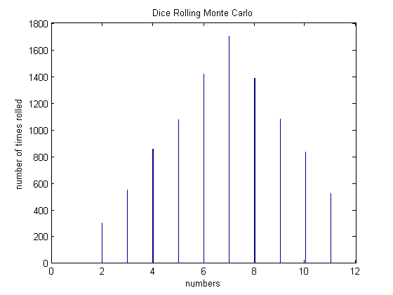
As expected, 7 is rolled the most amount of times.

One of the most basic Monte Carlo methods is the calculation of the value of pi. Look at the following picture, in which a black unit circle is inscribed into a white square: 

We know that the ratio of the area of the circle to that of the square is pi/4. If you need to prove this to yourself, simply divide the area of a circle by that of a square whose sides are twice the length of the circle’s radius. Now, imagine that you dropped a series of evenly and randomly distributed darts across the image. If you counted them, the number of darts within the circle should be about pi/4 times the amount of total darts dropped. It is much easier to simply count these darts than to try any other mathematical measurement. The following code allows us to simulate this scenario by randomly selecting coordinates within the image above. If the randomly selected coordinate has a value of 0, it is black and thus it is counted as having landed in the circle. Most of the trials yield a value of about 3.09, relatively close to pi. We believe that it is off because MatLab is not able to perfectly represent a circle as values in an array.

We then began to research basic option trading techniques. Option trading is a large field in the world of finance and uses computer simulations to traders. To start it was necessary to understand what an option is. The definition from Aswath Damodaran gives a simple, and concise answer: “An option provides the holder with the right to buy or sell a specified quantity of an underlying asset at a fixed price (called a strike price or an exercise price) at or before the expiration date of the option.” To fully understand this definition, it is critical to know that an underlying asset simply means a stock or a portfolio for our purposes.

Option trading typically uses binomial trees or the Black-Scholes method. The Black-Scholes method was published in 1973 and won the Nobel Prize in Economics in 1997, is a way of finding the end price of underlying asset given specified parameters. These parameters include: the strike price, K, the asset price, S, the volatility given by the symbol $\sigma$, the risk free interest rate, r, and the time until maturity T. The Black-Scholes model can be used for two different types of options, a put option and a call option. A call option provides the holder the right to buy the underlying asset at the specified strike price until the maturity date. Conversely, a put option gives the holder the right to sell an underlying asset at the strike price at any point until the maturity date.

For a less technical definition, lets say stock A is being traded for 10 dollars and you can purchase the call option for 2 dollars giving you the right to sell stock A for 10 dollars (the strike price). You believe that stock A will go up to fifteen dollars in a month, so you spend 200 dollars on 100 shares. Fortunately stock A has gone up to 20 dollars, so now you invoke your right to purchase 100 shares at 10 dollars each and then immediately sell stock A. This gives you a profit of 10 dollars a share giving a net profit of 800 dollars because we must take into account the 200 dollars you spent on the call option.  The Black-Scholes model is below:

(1)  

where

(2)  

and

(3)  

$N(d_1)$ is the standard normal distribution of $d_1$ and $N(d_2)$ is the standard normal distribution of $d_2$.

In our code we found the call option for a European option because it is slightly easier to code. For the parameters: $\sigma$ = .3, K=4, S=2, T=3, and r=.4 we get the call option price from the Black-Scholes model is .86415 and from the Monte Carlo method we get .86509. The Monte Carlo method provides a powerful way to check that our solution to the Black-Scholes model is correct. In our case we use an extremely large amount of random numbers. To check our example we encourage you to run our code, which can be downloaded at the link provided at the bottom of the page. Our code runs for the European Call Option and can be checked against: http://www.erieri.com/blackscholes.

A more advanced Monte Carlo method is used to solve an ising model that represents the spin states of electrons in a magnetic material. Here, we have defined the “isinggrid” to represent a system of interdependent spins. These spins naturally tend to align themselves in the same direction, and thus we have started with a ferromagnetic system in which all spins are aligned. We then simulate stochastic changes in the system that occur because of energy added by the temperature in a heat bath. As temperature rises, the greater there is that one of the spins will orient itself in a way that requires adding energy to the system. This is because the extra heat from the increased temperature supplies extra energy. We have also accounted for the spins at the edges of the grid by applying periodic boundary conditions that allow even spins on the edge to interact with four neighbors instead of two or three. We iterate through 11 temperatures in this example, calculating the overall magnetization for each one. This magnetization, M, is the average magnetization calculated 5000 times by the stochastic Monte Carlo process. If a spin flip results in a decrease in energy of the system, it occurs. If it increases the energy, the program generates a random number and then compares it to a parameter set by the temperature. Below is the average magnetization for each temperature that we tried:

As we can see, there is a very sharp drop off in Magnetization upon reaching a certain temperature, which we will calculate the exact value of by next week. This is a good step in our project, as it is important for us to get used to working with stochastic and semi-stochastic systems. Our financial models will involve similar sorts of ideas.

Link to our code: https://drive.google.com/folderview?id=0B01Mp3IqoCvhflF5azV4bHY2V0c3Vks0VXVyQkIxcnR4RmFaNDhVWEQtZGZSR2t6V2VWOHc&usp=sharing

New References:

1. The Black and Scholes Model: http://bradley.bradley.edu/~arr/bsm/pg04.html

2. Aswath Damodaran http://people.stern.nyu.edu/adamodar/pdfiles/option.pdf

3. Bruce Mizrach  http://snde.rutgers.edu/pubs/[42]-2010_Handbook.pdf

Sushant Mahat and Mohammed Abdelaziz

We created two functions to simulate the movement of dilute gas molecules in a container.

The first function initiates a grid of equally spaced points on which to initially place each particle. The function gives them random velocities and perturbs their initial position slightly from the equally spaced grid points.

The second function is a routine that updates the position of each particle at each time step. It determines the next position of each particle by determining the force acting on it due to all other particles in the box, based on the Lennard-Jones potential. The Lennard-Jones potential leads to a force that is large and repulsive at short distances, and attractive at larger distances. The repulsive force has been problematic, because two particles that encounter each other in the box get repelled at very large speeds, producing isolated points like those seen in our results below. If we can solve this issue, the results should be much more coherent.

Additionally, the simulation uses periodic boundary conditions, which we successfully implemented. A particle that “exits” one side of the box must return through the other side at the same velocity. The force calculations reflected this; two distances could be used to calculate the force: one that is between two points within the box, and another that takes into account the periodic boundary conditions. The shorter distance of the two was used to calculate each force.

We ran a calculation of 25 particles in a 10×10 box and obtained these results:

Once again, fixing the exponentially increasing forces is our top priority at this point; once we do so, we will be able to accurately calculate speed and velocity distributions of the particles in the box.

The two functions are attached as .pdf files.

Function 1: TheInitiator

Function 2: TheUpdater

A script was used to initialize variables, run the two functions, and plot the results.

EDIT (4/16/15)
The original *.m files have been uploaded and can be found here.

1. Introduction

The human body is an elastic and versatile model.  It can move muscles individually or in a systematic way in an instant. For our project, we are interested in exploring realistic projectile motion and human acceleration as it pertains to the human body.  While we often assume air resistance and spin to be negligible in Introductory Mechanics, as a way of simplifying our calculations, it is impossible to ignore their effects in competitive events like the long jump.  The additional drag force caused by a single misplaced limb can lead to a loss of centimeters on a jump.  This difference may indeed be negligible in the context of an Introductory Mechanics problem, but is everything to an athlete competing for medals and sponsorship.  For our project, we want to explore the effects of proper body position on the traveled distance in the long jump, in addition to exploring the negative effects of improper position.

2. Project Details

In order to do this, we believe we will need to devise a way of modeling the human body as a 3-dimensional object inside a larger 3-dimensional array representing space.  If we find it necessary later on, we can make the body as low profile as possible by modeling it as a stick figure.  We intend to impart initial conditions onto the object using the “Previous, Current, Next” template we have been using in our homework, to give the body an initial x and y velocity.  The experimentation will occur in the middle of the jump, where we will change the position of various limbs of the body (possibly through matrix multiplication, as is done in computer animation), and compare the results on the final jump distance.  Changing body position will both change the surface area profile of the body, changing the drag force, and change the body’s center of mass which may lead to spin in the face of wind.  We will draw examples of proper and improper form from the literature produced by top track and field coaches so that our program will be grounded in reality and have some practical value.

2. Motivation for Project

Track and Field and athletics in general have been major parts of both of our lives as, between the two of us, we have participated in basketball, volleyball, cross country, track and field, and swimming at a Varsity level.  Also, both of us have considered careers in the Health & Fitness Industry in the past, and are still interested in ongoing developments in the field. We are both interested in the underlying mechanisms that go into making the simplest, and most human tasks, such as walking, running, and jumping, as efficient as possible.  We also both competitive people and have spent years fussing over minute details to give us the smallest competitive advantage.  We are excited to see what we can accomplish now with our improved knowledge of physics and the powerful software at our disposal.

References (will add more at a later time)

Giordano, Nicholas J., and Hisao Nakanishi. “Chapter 2: Realistic Projectile Motion.” Computational Physics. 2nd ed. Upper Saddle River, NJ: Pearson/Prentice Hall, 2006. Print.

Kinematic Equations

Projectile/Range Equations

Timeline (subject to change depending on our work efficiency):

Week 1: The setup. Establishing the arrays, the initial variables and conditions.

Week 2: Run simple trial with one-dimensional object in two-dimensional space with air resistance.  Then second trial with a mass-less two dimensional object in 3-dimensional space.

Week 3: Two test trials with three-dimensional object in three-dimensional space, each with different body position.

Week 4: All trials complete, finalizing the written report and conclusion.

Goals and Sources

The goal of this project is to investigate some simple models of neural networks and memory, which are extensively used in cognitive science and related disciplines to model certain aspects of human brains.  Our project will follow Section 12.3 of Computational Physics by Giordano and Nakanishi, which draws on the Ising and Monte Carlo methods presented in Chapter 8.  This project will be attempting to investigate how to create this type of neural network model, how well it retrieves stored patterns depending on differing input patterns, how many patterns can be stored (and why there is a limit), how well the system functions when parts of the memory are damaged, and how the system learns new patterns.

Background

Chapter 8 introduces the Ising model, which is used to model magnetic substances and phase transitions with temperature changes.  The basics of this model are an array of spins, which are allowed only two orientations: up (+) or down (-).  These spins are connected to their neighbors so that they influence each other; when a negative spin is surrounded by positive ones, the flipping of the negative one to positive represents a reduction of energy.  The Monte Carlo method is used to search through the array, deciding if each spin should be flipped or not, according to its interactions with the surrounding spins, so that the energy of the system tends towards its minimum value.

+ + +           + + +

+  – +    →   + + +

+ + +           + + +

Using a 2-D array of completely interconnected Ising spins, a group of neurons can be modeled and investigated.  These neurons are very simplified, so that they are in only two possible states, firing (+) or not firing (-).  Patterns can be stored in these neural networks by formatting the connections between spins so that stored patterns correspond to energy minima compared to random patterns.  This is accomplished with Equation 12.18

where J_i,j is the connection array (which stores all the connection weights between the neuron spins), M is the total number of stored patterns, s_i (m) and s_j (m) are the configurations of spin i and j in stored pattern m.

Project Timeline

Week 1 (4/6 – 4/12)

We will begin by creating an Ising magnet program and learning the Monte Carlo method, following Chapter 8 and relevant examples closely.  This will set us up to be able to implement these tools on our neural network models later on.

Week 2 (4/13 – 4/19)

Next, we will create a simplified Neural Network, using symmetric connections and storing relatively few patterns, and test this network so that we are sure it functions as it should.  The beginning parts of Section 12.3 will be followed closely here.  In this process, we will figure out most of our code, in terms of creating neural networks, how the neurons are indexed, how to create patterns easily using for loops, how to store these patterns using Equation 12.18, etc.

Week 3 (4/20 – 4/26)

Here we will begin splitting up the topics for further investigation.  Routes of investigation include

a. How far away initial inputs can be from stored patterns while maintaining successful                     recall.

b. How many patterns can be stored in the neural network.  The book discusses the                           maximums associated with this type of neural network, but we will investigate why this                 limit exists, as well as what kinds of behaviors change around this limit.

c. How long (how many Monte Carlo iterations) recall of stored patterns takes.

Tewa will take charge of a and c.

Brian will focus on section b.

Week 4 (4/27 – 5/3)

We will continue to work on the investigations from week 3, and if we have time, we will progress to more complicated neural networks.  Some complications we can introduce are larger networks (and how the recall times might change), asymmetrically connected neurons (a more complicated weight connection matrix), and how further learning impacts the neural networks.

Week 5 (5/4 – 5/10)

We will continue any investigations we have left during this week, and begin writing up our results for final blog posts and presentations.

Week 6 (5/11 – 5/13)

We will finish up our blog posts and presentations, and present our results to the class.

An acoustic plane wave is defined much as you’d expect: as a “plane” of sound energy traversing a medium. When this wave encounters an object, there are several possibile outcomes:

1) Diffraction–the sound is “bent” around the object and its path is therefore altered;
2) Scattering–the sound is reflected off of the object and its path is thus altered;
3) Refraction–the sound passes through the object and its path is therefore altered due to a change in medium.

In this project I shall consider only diffraction and scattering, as the “object” I have chosen is a perfectly rigid, acoustically non-transparent sphere (i.e. sound cannot pass through it). In practice, it is seen that diffraction occurs for high wavelength (low frequency) sound only, and as frequency increases, scattering becomes the dominant phenomenon.

Like any wave, there is a wave equation dictating the propagation of an acoustic wave. Its solution is, however, quite complicated (especially in the presence of objects/barriers), and although analytical solutions exist for diffraction and scattering on a sphere, its components, which require complex functions such as Spherical Bessel and Hankel functions and their derivatives, whose values cannot be precisely (analytically) determined using computational methods, and which therefore must be approximated much like we approximated the solutions to differential equations using the Euler, Runge-Kutta, or similar methods.

For the sake of illustration the acoustic wave equation in three dimensions is:

Notice that this is a 2nd order differential equation the likes of which we have handled in class.

The layout of the project is this (in order of importance):
1) to use the acoustic wave equation to numerically solve the problem of diffraction (low frequencies) and scattering (high frequencies) of the wave on the surface of a rigid sphere;
2) to compare this result to the analytical results available;
3) to provide a visual or graphical representation of the phenomena;
4) to discuss error propagation in numerical method and the method by which the Spherical Bessel and Hankel functions described earlier are approximated;
5) to, if possible, discuss the spherical harmonic decomposition of sound on the surface of the sphere, which provides a rigorous basis for accurately modeling the sound up to a certain frequency.

This last point also requires the evaluation of integrals (in a way analogous to that of Fourier Transforms in 2D), which by the nature of computation are impossible to solve perfectly using numerical methods, but must be approximated as sums. If I am able to include this last point, I will also discuss the method of approximating the integrals.

Physics of Musical Instruments Project Plan

Greg Cristina, Teddy Stanescu

Objective:  Explore the physics behind the sound of different musical instruments; vibrations through different mediums and the frequencies they create. We will be looking to experiment with these three musical instruments:

1. Guitar (a plucked string)
2. Piano (a hammered string)
3. Drum (a hammered membrane)

Chapter/Section(s) of Focus: We will focus on theory and use equations from Chapter 11 in the class text (Giordano), specifically sections 11.1, 11.2, and 11.4.

Overview: We want to model each of these 3 instruments in Matlab, using the computational methods and equations provided in the text.  These models will consist of the physical behavior of the instruments, such as (x,y,z) displacement of a string/membrane at a given time t and the frequencies/harmonics (overtones) they produce given specified initial conditions.  From here, we will take advantage of Matlab’s ability to read and extrapolate data from audio files by mimicking our theoretical scenarios modeled in Matlab as a physical test, using the actual instruments, keeping as many initial parameters as possible constant.  We will record the sound produced by the instruments using a microphone and recording software (audacity/reaper), import to Matlab, and compare the recorded data to the data calculated through the computational methods.

Experimentation:  For the guitar string, we will pluck the string at different distances from the bridge.  For the piano string, we will strike the string with different strength forces from the hammer.  These changes in how the instrument is played are shown in the text to yield different frequencies and harmonics, and we will further investigate this phenomenon.  The drum will be the biggest challenge to experiment with because there is no direct example in the text.  However, it covers many methods that we will modify and test such as relating the force of a guitar or piano string on the soundboard to the frequency it produces.  Also, the text has a banjo example of how a wave on a string affects a membrane and the frequencies they produce, which is similar to the two heads of a drum interacting with each other to produce a sound.  Using knowledge gained from experimenting with the guitar and piano strings, we will investigate drum membrane physics and attempt to model in Matlab, if model is successful, a recording with be made and compared.

Sources used (as of now):

–Computational Physics, Nicholas Giordano

-more to come if necessary

Timeline:

Week 1 – Model guitar string in Matlab, and test at different distances from bridge.

Week 2 – Model piano string in Matlab, and test different hammer forces

Week 3 – Record guitar and piano string, analyze and compare with Matlab calculated data

Week 4 – Drum experimentation

Week 5 – Organize data in a presentable manner, fix any errors in data analysis

The goal of this project is to extract 2 relevant measures stemming from an EMG or nerve signal, the peak cycle amplitude and cycle duration. These two measures as demonstrated in several academic papers in a variety of model organisms, are the measures most consistently correlating with a muscle response. An idealized nerve spike train signal appears as repeating spikes, whose amplitudes and frequencies vary according to the action at hand. However, this method has several issues with both execution and correlating to the physical model. Primarily, depending on the scenario at hand, there will be constant low level nerve activity corresponding to maintaining a given muscular contraction, this activity is extremely difficult to distinguish from noise.

The relevant measure will be quasi-linked in the code, with the program measuring nothing, peak amplitude, or amplitude and cycle duration depending on the magnitude of the signal from the EMG. However, prior to any signal extraction, the program will run a Fourier transform (due to software, hardware  and time restrictions, this iteration will likely store data in bins and process after each bin, as opposed to continuous measurement), excise the largest and most common noise signals (such as 60Hz noise emanated by  many electronic devices), and transform the spectrum back as a rectified signal. The system will not update (essentially being in a resting state), when there are no peaks above a noise threshold for a given duration. This  first threshold, determined by measuring the mean peak magnitude of noise registered by the EMG that is not connected to a live test subject will provide a lower limit on the kinds of information that the program will save. Above this first threshold, the program will record the peak amplitudes of the EMG signal. This can be used to keep the robotic agent at some non-resting state, without any motion. A second threshold, determined by the difference of magnitude between 2 measured peaks, will incite contraction in the arm. Once this threshold is passed, the program will measure all peaks for the cycle, and the the cycle duration (start and finish determined by the difference between each contracting peak and the last pre-contraction peak). The cycle duration will control the length of the contraction as determined by a scale elsewhere in the project, and the highest peak will be used to set the speed of the robotic arm’s motion.

Each signal will correspond to a single robotic degree of freedom, such that this program will be repeated uniquely for each EMG channel. A major limitation at this initial stage of design is available processing time, as the time required to process each signal will likely exceed the time that the biological agent would execute the same motion. As such, this initial setup will have signals taken at a different time than processing. This iteration will be written in Matlab, although later versions of the code will likely be run elsewhere.

Timeline:

Week 1: Execute background research, create an architecture on paper to use as a blueprint for the actual program

Week 2: Write the code for the Fourier transform, bin size to be determined later, harvest the noise signal and find the lower threshold for the data acquisition program

Week 3: Write the code to gather the relevant signals and set the thresholds and bin sizes depending on processing time.

Week 4: Finish writing/modifying code, prepare presentation and write up report for the project.

Sources:

TBD (There are several from the thesis list, I just have to select which ones I am going to use and possibly gather a few others)

The goal of this project is to investigate two problems in celestial mechanics for which a computational solution is quite valuable: the precession of the perihelion of Mercury and Kirkwood gaps, both found in Chapter 4 of Computational Physics by Giordano and Nakanishi. In the case of Mercury, the precession can be calculated analytically thanks to general relativity, but a computational solution is easier to obtain. Giordano and Nakanishi describe the process of obtaining the rate of precession, keeping in mind that this variable must be adjusted for practical computation times (that is, not 230,000 years), using the force law predicted by general relativity:
F_G ≈ (G M_S M_M)/r^2 (1+a/r^2 ),
Where M_M≡mass of Mercury, M_S≡mass of Sun ,a ≈1.1 ×〖10〗^(-8) 〖AU〗^2.
Part of the project will be to compare different computational methods for analyzing this procession, particularly the Euler-Cromer method and Runge-Kutta (which uses the Euler-Cromer method to update its values). Using a two-body system simulation, the value for rate of procession can be found by varying until it matches expected, observed rates.

The second computational problem covered is one for which an analytical solution is difficult, as the system is considered chaotic. In our solar system there are certain “gaps” in orbital radii from the Sun at which there are far fewer asteroids. Numerically it can be found that these gaps occur at certain resonances with Jupiter’s orbit, such as 2/1, 5/2, 7/3, etc. Running a simulation to find Kirkwood gaps and investigate asteroids’ paths near these gaps first involves construction of a multi-body model, at least a two-body system for the Jupiter and Sun, and for more accuracy (if time permits) a three-body system along with the Earth. Luckily the magnitude comparison between Jupiter and an asteroid makes their mass insignificant, meaning their gravitational force can be excluded from the simulation without much effect on accuracy of the program. An analysis of the asteroid’s orbits will also naturally include a discussion of chaos, described in Chapter 3 of Giordano and Nakanishi.

Timeline:
Week 1: Continue background research on physics and computational methods of analysis, write code for precession of perihelion of Mercury, begin (and hopefully finish) writing code for 2- or 3-body system in Kirkwood problem
Week 2: Adjust solar system model to include simulations of asteroids, their paths/orbits, finish all code, begin gathering data.
Week 3: Finish gathering data, finish all research, comparison to actual observed/computer values from literature sources.
Week 4: Finish data analysis, write-up for project, prepare presentation.

Sources:
Computational Physics, Giordano and Nakanishi, Chapters 3 & 4.
Mercury’s Perihelion from Le Verrier to Einstein, N.T. Roseveare.
Chaotic Dynamics in the Solar System, J. Wisdom.

Purpose and Goals

One purpose of this course is to explore the use of computational methods to find solutions to otherwise difficult analytical problems. The 3-body system is a prominent example. It is relatively straightforward to solve the equations of motion of a 2-body problem analytically, but far more difficult to do so for 3 bodies. The introduction of computational methods have allowed for fairly straightforward ways of analyzing 3-body motion.

A prominent example is that of the Sun, the Earth, and Jupiter, bound by the force of gravity. Since Jupiter is about 0.1% of the solar mass, it is the next biggest influence on Earth’s orbit in the Solar system. Using computational methods to analyze Jupiter’s effect would be far more efficient. We seek to create a model of the orbits of the Earth and Jupiter bound to the sun–and interacting with each other–via the inverse square law of gravity.

For this project we plan to make use of sections 4.1 and 4.4 in Giordano’s book. 4.1 outlines a method for calculating the motion of a planet orbiting the sun, whereas 4.4 opens the model to include Jupiter. The program will generate position data for each planet given their acceleration due to gravity, using the Euler-Cromer Method to approximate each new position based on this acceleration. We will start with a simplified model, with the Sun fixed to the origin, then graduate to a true 3-body model, where the origin would be fixed at the system’s center of mass.

Physics

We start with Newton’s Law of Gravitation, where Ms is the solar mass, Mp is the planet Mass, Fp is the gravitational force experience by the planet due to the Sun, and G is the gravitational constant:

Fp=G*Ms*Mp/r^2

Solving for acceleration (given Newton’s 2nd Law: Fp=Mp*a), or d^2x/dt^2:

a=G*Ms/r^2

This solution for acceleration is a second order differential equation, appropriate for use with the Euler Cromer Method.

Foundational Code (Routines provided in Giordano)

Planets: A routine to model the orbit of a planet around the sun as described by the inverse square law of gravitational force, with the sun at the origin. The Euler-Cromer method is used to approximate position. The Euler Method by itself would not be sufficient, as with all oscillatory motion it would introduce energy into the system and the planet would move away from the Sun. The Euler-Cromer Method guarantees a conservation of energy over one orbit.

Jupiter-Earth: Expands the above system to model Jupiter and Earth orbiting the sun. This method will also use the Euler-Cromer method for the same reasons. The suns mass will affect the orbits of the other two planets but the sun itself will sit at the origin of the system and not move.

True 3-body: This model is similar to the Jupiter-Earth model but instead uses the center of mass of the system as the origin. This model will be used when we are altering the mass of jupiter to be close to that of the sun, therefore causing changing orbits for each planet in the system. In this case, we want the sun to be able to move to better describe the full motion.

Initial Resources

http://astro.geo.tu-dresden.de/~klioner/celmech.pdf

http://arxiv.org/pdf/astro-ph/0411043v1.pdf

http://www.iumj.indiana.edu/docs/27030/27030.asp

Computational Physics, Giordano and Nakanishi. Sections 4.1 and 4.4.

Timeline

Week 1 (4/6-4/12)

During the first week we hope to work on organizing sources and solidifying understanding of background materials and physics. We will also use this week to read the Giordano text to begin understanding the setup of the MATLAB routines. We will begin writing the code for the Planets routine. This routine does not directly inform the 3-body problem but is the foundational code for the project. For the entire first week we will split the workload together since this work constitutes the base understanding of our project.

Week 2 (4/13-4/19)

Since the Planets routine should be well defined and operational by this week, we will use this time to finish off the other routines. This should be manageable since both the Jupiter-Earth and True 3-body routines are derivations of the Planets routine. Nadav will work on the Jupiter-Earth model while Matteo tackles the True 3-Body routine. This week will mostly be coding based, as we hope have all models complete by this time.

Week 3 (4/20-4/26)

By now, all routines should be complete. We will use this week to explore the implications of our models. This exploration will consist of multiple demonstrations of the effects of the changed mass of Jupiter on the system and will also include qualitative conclusions. We will also begin to work on writing up our results, with each of us taking charge of specific simulations.

Week 4 (4/27-5/3)

This final week will consist of finishing up our written results and finalizing the report. We will also leave space here for potential further exploration of our system, given appropriate time. Possible extensions include adding in another body to the system or analyzing in more detail the stability of orbits (Section 4.2, Giordano).

Through random system analysis, I would like to determine both a trend for 2D motion between 2 locations and how altering specific real world variables can change this trend. I will be using Chapter 7 of the class text the most for the basic bulk of the code. However, I will be developing novel aspects for my code in order to simulate certain variables within the random journey.

This epic journey will be through the weary eyes of a Vassar student struggling and stumbling (strumbling, if you will) their way back from a long and alcohol filled night. We find this student past inebriation and past wasted: at this point, the poor soul is taking random steps in random 90 degree turns back to their room. They even fall down from time to time. However, there is hope yet! They have a friend with them that will guide them back to their dorm with a gentle push from time to time. How long will it take them to make it back?

The random variables listed above (and I will probably find some more) will be simulated by additional conditions in the MATLAB code and represent real and mathematic aspects of random motion. I will analyze their effects and relative weights of each via multiple graphs that will attempt to find a trend or average number of steps for a certain distance. I would then like to increase the distance gradually in order to find an expression for displacement traveled and the number of steps required.

I would like to present my data as scatterplots of steps required. By adding additional variables during the walk, I can compare their individual effects. In addition, I can watch the effects the relative weights each variable has on the outcome. For example, does a higher rate of falling down change the outcome more than less drift induced from the friend? Toying with relative weights can also make the journey more realistic.

This project allows me to use statistical analysis and probability to map the path of an independent data point with variables imposed on it. This introduces a lot of variance in the data and my largest stumbling block (get it?) will be extracting concrete data from this. Data might also be difficult to extract with pure random motion at long distances. This project also leaves different relationships between variables wide open so I can qualitatively compare variables if concrete data is weak.

Week 1

Writing the bulk of the code and determining whether there is a trend without drift.

Week 2

Implementing additional variables and watching their affect on steps required

Week 3

Data compilation and figure creation

Week 4

Hopefully I’m done around here but if not, I might add another variable to the mix and see how it affects the steps required to reach the destination. Data compilation might spill over into this week too.