Category Archives: Spring 2012

Preliminary Results

I modeled the effect of $\bigtriangleup k$ using the equation:

(1)   \begin{equation*} I_{3} = \frac{512\pi^{5}d^{2}I_{1}I_{2}}{n_{1}n_{2}n_{3}\lambda^{2}_{3}c}L^{2}\frac{\sin^{2}(\frac{\bigtriangleup kL}{2})}{(\frac{\bigtriangleup kL}{2})^{2}} \end{equation*}

2.2.20 Nonlinear optics Robert W.Boyd

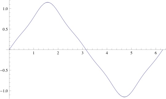
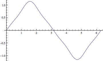
This can be simplified to $I_{3} = I_{3}(max)\frac{\sin^{2}(\frac{\bigtriangleup kL}{2})}{(\frac{\bigtriangleup kL}{2})^{2}}$

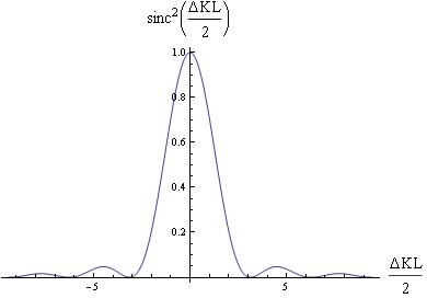
Fig 2.2.2 Nonlinear optics Robert W.Boyd

Link to mathematica code https://vspace.vassar.edu/tasanda/sinc.nb

It shows the harmonic generation output as a function of the phase match $\bigtriangleup k$ when $\bigtriangleup k \sim 0$

Link to mathematica code https://vspace.vassar.edu/tasanda/Manipulation.nb

This model shows the effect of superposition of waves and explains why intensity is largest when $\bigtriangleup k=0$

Deriving Efficiency

Solving the general wave equations for the two frequencies $\omega_{1}$(incident) and $\omega_{2}$(Second harmonic) we obtain coupled-amplitude equations.

(2)   \begin{equation*} \frac{dA_{1}}{dz}= \frac{8 \pi id \omega^{2}_{1}}{k_{1}c^{2}}A_{1}A_{2}e^{i\bigtriangleup kz} \end{equation*}

(3)   \begin{equation*} \frac{dA_{2}}{dz}= \frac{4 \pi id \omega^{2}_{2}}{k_{2}c^{2}}A^{2}_{1}e^{i\bigtriangleup kz} \end{equation*}

2.6.10, 2.6.11 Nonlinear optics Robert W.Boyd

Where $\bigtriangleup k = 2K_{1}-k_{2}$ is the wave vector mismatch. Integrating these equations gives us

$A_{1}=(\frac{2\pi I}{n_{1}c}) u_{1}e^{i\phi_{1}},       A_{2}=(\frac{2\pi I}{n_{2}c})u_{2}e^{i\phi_{2}$

2.6.13, 2.6.14 Nonlinear optics Robert W.Boyd

The new field amplitudes $u_{1}$ and  $u_{2}$ are defined such that $u_{1}(z)^{2} + u_{2}(z)^{2} = 1$(conserved normalized quantity). Next we introduce a normalized distance parameter

$\zeta=\frac{z}{l}$     where      $l=(\frac{n^{2}_{1}n_{2}c^{3}}{2\pi I})^{\frac{1}{2}}\frac{1}{8\pi \omega_{1} d}$

2.6.18, 2.6.19 Nonlinear optics Robert W.Boyd

$l$ is the distance over which the fields exchange energy.

$\frac{du_{1}}{d\zeta}=u_{1}u_{2}sin\theta$ and $\frac{du_{2}}{d\zeta}=-u^{2}_{1}sin\theta$.

2.6.22, 2.6.23 Nonlinear optics Robert W.Boyd

If we assume $cos\theta=0$ and  $sin\theta=-1$ the equations simplify to  $\frac{du_{1}}{d\zeta}=-u_{1}u_{2}$   and   $\frac{du_{2}}{d\zeta}=u^{2}_{1}$

2.6.31, 2.6.32 Nonlinear optics Robert W.Boyd

The second equation can be written as $\frac{du_{2}}{d\zeta}=1-u^{2}_{2}$(from conservation).

Hence $u_{2}=tanh(\zeta+ \zeta_{0})$. Initially we assume there is only the incident beam and no harmonic generation hence $u_{1}(0)=1, u_{2}(0)=0$. Therefore $u_{2}= tanh\zeta$ and  $u_{1}=sech\zeta$. Plotting these two equations below shows that incident waves are converted into the second harmonic.

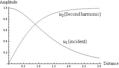
Fig 2.6.3 Nonlinear optics Robert W.Boyd

Link to mathematica code https://vspace.vassar.edu/tasanda/u1u2.nb

The efficeincy $\eta$ for the conversion of power from incident wave $\omega_1$ to $\omega_{2}$ is

(4)   \begin{equation*} \eta= \frac{u^{2}_{2}(L)}{u^{2}_{1}(0)} \end{equation*}

2.6.43 Nonlinear optics Robert W.Boyd

From the diagram it seems like increasing the medium length will increase the amplitude but doing so is not practical. Generally a higher pump intensity leads to a larger $\eta$ except to the limit of very high conversion efficiency.

Taking an example of a medium of 1cm length, the efficiency equals $tanh^{2}(1)$ which is $58\%$


Share

Intro To Preliminary Results

As it turns out, the equations for magnetic fields and forces that I was hoping to plot in Mathematica are too complicated for Mathematica to handle. I am unsure whether this drawback just applies to my Student version of Mathematica, or if my personal computer is to blame. However, I took a slight deviation to begin my studies with a simpler equation to model, the equation for the magnetic force between two plates of some finite area, given by:

(1)   \begin{equation*} F_{B}=\frac{B^{2}A}{2\mu_{0}} \end{equation*}

where B is the magnetic flux density (magnetic field strength) at a given distance above the bottom magnet, A is the common area between the two plates, and \mu_{0} 
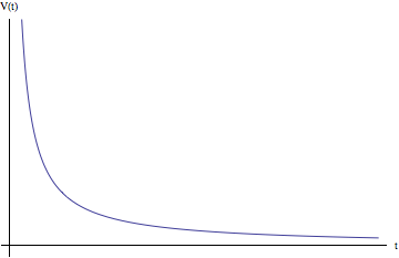
is the permeability of free space. In order to easily visualize this effect, I generalized the magnetic flux density by replacing it with a constant multiple times the inverse of distance cubed (which is the relationship between magnetic field strength and distance), producing the following graph in Mathematica:

Clearly, the force falls off extremely quickly with respect to distance, so I am expecting my other graphs to have a range of many fractions of a meter. This outcome is exactly as I would expect (ignoring any fringing effects near the edges), since the magnetic force between the two magnets decreases rapidly with distance; in my future calculations, I will expect the force on the top magnet to increase as the two get closer together, and decrease as the magnets separate, hopefully leading to a steady distance between the two over time. As soon as I can get Mathematica to accept my more complicated equations and graphs, I will post them.

Share

Preliminary Results

First, to set up my initial findings, I will show a comparison of a sine wave vs the Fourier Transform that I used to approximate a triangle wave.  Note how the transform is much closer to a linear function than the sine wave.

The link to the mathematica code for both of these can be found at the bottom of the page.

Now I will move on to the work that I have done with my triangle wave.  The first thing that I examined, as it seemed the most interesting, was the relative velocity $\omega_s – \omega_r$ which I simply called $d$ in my simulation.  This seemed the most interesting off the bat as it’s one of the only variables that appears both inside the sine term, and as a factor of the total expression’s amplitude.  Increasing the $d$ value on my plot of $B$ over a single cycle shrank the period dramatically but also increased the amplitude, yielding a much larger number of much skinnier spikes in $B$, as can be seen below.

It appears that the key is finding the balance between number and size of spikes (higher or lower relative rotation frequencies) that yields the highest overall total $B$, and thus the highest induced emf.  To this end, I tried to plot the integral of the absolute value of $B$ (the absolute value being introduced to account for all negative and positive values of $B$ as both contribute to the total emf) against an increasing $d$.  Unfortunately, Mathematica is unable to process this computation.  I have attempted to plug in points in between $d = 1$ and $d = 10$ to pinpoint a local max, or find that it continues to increase, but mathematica is being uncooperative with this computation as well.  Now that I know what exactly I’m looking for (in this vein at least), getting to it should not be too difficult.  For my next post, I will attempt to solve this problem using a 3-dimensional graph to include both $d$ and $t$ (the variable that cycles the sine waves) as variables.


Mathematica code for the all images:  continuous plots, data and discrete plot, sine and triangle wave.

Share

Preliminary Data

A very simplified way to look at LCD screens is to break them down into their most critical components. These would be the backlight, polarizer layer, liquid crystal layer, color filter (if it’s a color LCD screen), and second polarizer layer (there can be more than two polarizer layers, but we will visualize how the LCD screen works using this simple model).

What happens within these screens is that a voltage is applied to the liquid crystal layer, causing the liquid crystal to twist. Between the polarizer layers and the twisting liquid crystal, the intensity of the backlight is decreased in each cell depending on the voltage applied and, thus, how the liquid crystal twists, causing polarization effects. Color emerges as a result of red, blue and green color filters. In each pixel of the screen, different intensities of red, blue, and green will create the colors we perceive.

Liquid crystal cells (LC cells) act as wave plates (also known as retardation plates). Wave plates change the polarization of the incident beam.

If we have N equal the number of wave plates, then an LC cell will have a Jone’s matrix that looks like…

MLC = MN ….M3 M2 M1

An example of a corresponding Jone’s vector model of a wave plate would be this:

(1)   \begin{equation*} M_\delta = \dfrac{1}{\sqrt{2}}\left[ \begin {array}{ccc} e^{j\delta}&0\\ \noalign{\medskip} 0&e^{-j\delta} \end {array} \right] \end{equation*}


Where delta stands for the phase delay.

I am having trouble figuring out how to work Mathematica, but what I want to do is to create a graph that will show how each polarization has a different minimum, total twist angle, and retardation, and to particularly show this for viable commercial numbers.

The different twisting of the liquid crystal, as I said before, greatly affects what we see on the screen. When the twisting angle is much smaller than the double refraction (birefringence), the light is linearly polarized. While if the twist angle is large in comparison to the double refraction, the light in the cell will be circularly polarized.

The transmission of the LCD can be modeled using variations of the Gooch and Tarry formula:

(2)   \begin{equation*} T=\dfrac{1}{1+u^2}\left\{u^2+cos^2\beta{d}\right\} \end{equation*}


I am going to continue to play with this equation in order to look at how transmission is altered and when and why it peaks as well as what typically produces the best results for commercial usage.

Since PDP and CRT screens do not rely on polarization in order to adjust the intensity of light, I intend to investigate EMI shields and how they contribute to PDP screens to be of a better picture quality than CRT screens.

References:

Angelov, T.,  et. al. “High Temperature Formation of Polymer-Dispersed Hydrogen Bonded Liquid Crystals.” Journal of Optoelectronics and Advanced Materials Vol 7.1 (2005): 281-284.

Collett, Edward. Field Guide to Polarization. Washington: SPIE Press, 2005.

Gooch, C.H. and H.A. Tarry. “The optical properties of twisted nematic liquid crystal structures with twist angles less than or equal to 90 degrees.” Applied Physics Vol. 8(1975): 1575-1584.

Share

Preliminary Results

The equations and plots I present here all consider a positive point charge with constant velocity v starting at the origin at time t = 0, and moving along the z axis. They derive from Griffiths example 10.3.

First we take the simplest case. If we consider the electric potential at the origin (r = 0) over time as the particle moves upward, we have:

(1)   \begin{equation*} V(t) = \frac{qc}{\sqrt{(c^2t)^2+(c^2-v^2)(-c^2t^2)}} =\frac{q}{vt} \end{equation*}

Note that the potential does not depend on the speed of light. This is due solely to the fact that the particle begins moving from the same point we are considering; the speed of light is only of import when at t = 0 there is some electromagnetic information which has not yet reached the point we are considering, for then we need to know how fast that information is traveling.

The above is a familiar graph where V is proportional to the reciprocal of t. As we can see, the origin’s potential is infinite as time t = 0 (because the point charge is located there), and as the charge moves away along the z axis the potential falls off to zero asymptotically.

The next equation modifies Griffiths 10.42. We express the dot product in the denominator using cosine, expressing the desired angle in terms of x, y and z.

(2)   \begin{equation*} V = \frac{qc}{\sqrt{\left(c^2t-\frac{vz\sqrt{x^2+y^2+z^2}}{x^2+y^2+z^2}\right)^2  +\left(c^2-v^2\right)\left(x^2+y^2+z^2-c^2t^2\right)\right]}}          \end{equation*}

The original Mathematica code for the following animations allows many different values of z and t, but I’ve posted two possible configurations below. The first is where z is positive, so the charge passes us at some point (hence the potential grows larger at first), and the second is the special case where z is zero, which describes the potential of the xy plane over time.

Note: in the first animation there is an asymmetry in the electric potential near the origin that becomes evident at times where the potential grows large. However, the x and y variables in 10.42 are completely interchangeable, and I am unable to come up with a physical or mathematical argument for this. It may indicate a problem with Mathematica’s sampling rate near large function outputs.

Similar to the graph above the potential in both animations decreases very quickly at first, then more slowly. We can write the denominator of Griffiths 10.42 as a polynomial in t:

(3)   \begin{equation*}           \sqrt{ (v^2 c^2)t^2- (2c^2\vec{r} \cdot \vec{v})t + c^2r^2 -v^2r^2+( \vec{r} \cdot \vec{v})^2           \end{equation*}

Since polynomials are dominated by their leading term for large values, the denominator of 10.42 is approximately t for large values of t. Thus for large values of t, the electric potential decreases in a way similar to the origin case (where V is proportional to the reciprocal of t), but in general will decrease faster. Considering the origin is a subcase of considering the entire xy-plane; this means it represents a special sort of minimum: one where the electric potential will fall off more slowly than anywhere else! This makes sense in terms of the physical situation: at any time, the point in the xy-plane closest to the point charge is the origin. The surprising part is how much that makes a difference. Whereas for the origin case the electric potential decreases proportional to the 1/t, for the rest of the xy plane  it decreases proportional to 1/t^2.

The magnetic vector potential due to a point charge with constant velocity should also go to zero for large values of t, but I’m having trouble getting my current models to reflect this. Vector models and animations for this are to come, as well as for the event horizon problem presented as 10.15 in Griffiths.

Share

As discussed before, I will be looking at how magnetic fields induce currents in wire coils. The setup I have chosen to focus on has magnets passing over a stationary coil as shown below.

For the purpose of my diagram, we see a north, a south, and another north pass over the coil. Each magnet has a radius of 2cm and 1cm gap between them. This is one of the few things that is not variable in my animation.

The first thing I will concern myself with is producing the equation for the magnetic field. I will start with the following equation:

(1)   \begin{equation*} B=\frac{\mu _{0}}{4\Pi }\frac{2\mu^{3}}{d^{3}} \end{equation*}

After plugging in the constant for \mu_{0} and scaling it to get millitesla I get the equation:

(2)   \begin{equation*} B=\frac{2\mu^{3}}{d^{3}}*10^{-4}\;\;\;mT \end{equation*}

Aha! I have the magnetic field dependent on distance. This is great, but I am more interested in having one dependent on time. Here is where the heavy lifting comes in. I will now assume that all of my other variables are constant, with the exception of time. Time should only effect one thing with the magnetic field, and that is the direction of the field. This changing magnetic field is the exact effect that we need to make induction work. Since the only change is the direction we know that the range of the field is -B to B. This means that we need a function that oscillates linearly from 1 to -1 and then multiply our equation derived for B by this new oscillating function.

The reason I chose a linear function, is because as one magnet moves away an opposite one moves in. I am going to make the assumption that when the north facing and south facing magnets are equidistant from the center of the coil, the magnet field within is zero. What I hope to achieve is a function that will linearly rise and fall from 1 to -1, and what better way to do that than with a triangle function.

The equation for this triangle function is:

(3)   \begin{equation*} \frac{4}{p}\left ( \left ( t+.5 \right ) -\frac{p}{2}\left \lfloor \frac{(2t+1)}{p}+.5 \right \rfloor\right )\cdot (-1)^{\left \lfloor \frac{(2t+1)}{p}+.5 \right \rfloor} \end{equation*}

Where p is the period, and the bottom side brackets \left \lfloor floor \;fn \right \rfloor are floor functions.

As stated earlier the magnets have a radius of 2cm and separation distance of 1cm. Since this is constant we know that the distance between the peaks of the triangle function has to be 10cm (2+1+4+1+2) using the equation v=\frac{d}{t} we can say that p=\frac{.1m}{v}.

Using this new definition of p, (and assuming v is constant) we get the following equation:

(4)   \begin{equation*} 40v\left ( \left ( t+.5 \right ) -\frac{.05}{v}\left \lfloor \frac{(2t+1)v}{.1}+.5 \right \rfloor\right )\cdot (-1)^{\left \lfloor \frac{(2t+1)v}{.1}+.5 \right \rfloor} \end{equation*}

which in turn leads us directly into our new equation for B:

(5)   \begin{equation*} B(t)=\frac{2\mu^{3}}{d^{3}}10^{-4}\cdot40v\left ( \left ( t+.5 \right ) -\frac{.05}{v}\left \lfloor \frac{(2t+1)v}{.1}+.5 \right \rfloor\right )\cdot (-1)^{\left \lfloor \frac{(2t+1)v}{.1}+.5 \right \rfloor} \end{equation*}

We have successfully found B as a function of t!

Now we have the magnetic field some distance from the magnet. The next step is to find the flux. Since in my diagram the magnet is larger than the coil (and at most the same size) I will only worry about the coil’s area. I also have no pitch on the magnets or wire, so angle is irrelevant and will be ignored from here on. Using the following equation:

(6)   \begin{equation*} \Phi _{B}=\int B\cdot da \end{equation*}

we find:

(7)   \begin{equation*} \Phi _{B}=\frac{2\mu^{3}}{d^{3}}10^{-4}\pi r^{2}d_{w}N=Nd_{w}\frac{2\pi r^{2} \mu^{2}}{d^{3}}10^{-4} \;mW \end{equation*}

Where d_{w} is the diameter of the wire and N is the number of turns.

Since one of the main goals is to find the emf, we need to find \Phi_{B} with respect to t. Luckily, we did most of the work already when we derived B(t). The new equation reads:

(8)   \begin{equation*} Nd_{w}\frac{2\pi r^{2} \mu^{2}}{d^{3}}10^{-4}40v\left ( \left ( t+.5 \right ) -\frac{.05}{v}\left \lfloor \frac{(2t+1)v}{.1}+.5 \right \rfloor\right )\cdot (-1)^{\left \lfloor \frac{(2t+1)v}{.1}+.5 \right \rfloor} \;mW \end{equation*}

For simplicity I will quickly denote C=-Nd_{w}\frac{2\pi r^{2} \mu^{2}}{d^{3}}10^{-4}40v

We can now move along to the emf!

(9)   \begin{equation*} \varepsilon = -\frac{d\Phi_{B}}{dt} \end{equation*}

Plugging in our absurdly long equation for the flux, we get:

(10)   \begin{equation*} \varepsilon = C\frac{d\left ( \left ( t+.5 \right ) -\frac{.05}{v}\left \lfloor \frac{(2t+1)v}{.1}+.5 \right \rfloor\right )\cdot (-1)^{\left \lfloor \frac{(2t+1)v}{.1}+.5 \right \rfloor}}{dt} \end{equation*}

How would you take a derivative of this triangle function with respect to t? Well, you can’t. At least, I can’t, but what I can do is find an adequate approximation. I know that the positive slope is .025v^{-1} 
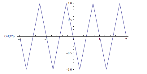
and the negative slope is -.025v^{-1}. From here I can ascertain the derivative simply by finding a function that flips back and forth between those two values every .05v^{-1}, which should look like a square function.
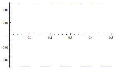
The equation for which is:

(11)   \begin{equation*} .025\cdot sgn [sin(\frac{\pi t}{.05v)}] \end{equation*}

Where the sgn function simply takes all positive values and makes them 1 and all negative values and makes them -1. This gives us an emf of:

(12)   \begin{equation*} \varepsilon = C \cdot .025\cdot sgn [sin(\frac{\pi t}{.05v})] \end{equation*}

and an induced current of

(13)   \begin{equation*} I(t)=\frac{\varepsilon}{R}=.025C \frac {sgn [sin(\frac{\pi t}{.05v})]}{R} \end{equation*}

HUZZAH!!

Share

Preliminary Results

The magnetic field inside an NMR spectrometer is generated by a superconducting solenoid.  The solenoid is cooled by a three-layer cooling system.  The outer layer is one of liquid nitrogen at 77K.  The middle layer is an evacuated cavity that prevents heat conduction by air.  The innermost layer contains the solenoid submerged in 4K liquid helium that is kept below atmospheric pressure.  Initially, the magnetic field in an NMR will not be homogenous because of interferences resulting from the magnetization of the sample, and environmental interferences like iron or other metals used in construction.

Initial NMR Magnetic Field

Sample NMR Starting Magnetic Field

Note the somewhat ordered field that already exists in the Z-direction.  This is what the initial field looks like most of the time:  the inhomogeneities are a complex function in three dimensions.  In order to make the magnetic field homogenous, it is modified using the shim system. The shim system is a series of uncooled, current carrying coils that generate fields in all three directions.  Each coil attempts to create a field with a function that precisely cancels the imperfections.  Numerous simple 3-D functions like X, Z, XY^{2}, Z^{2}, Z^{3}, Z^{4}, XZ, YZ, and X^{2}-Y^{2} 
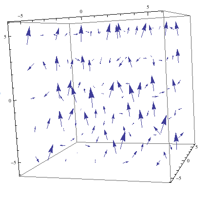
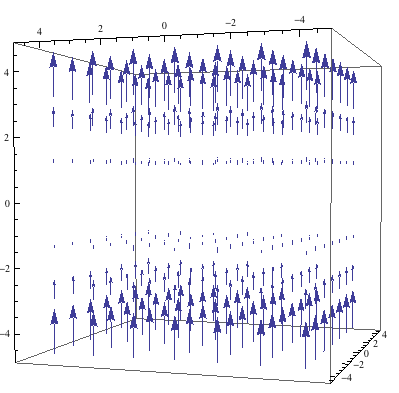
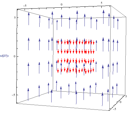
are available to add to the magnetic field created by shimming.  Each set of coils creates a magnetic field gradient in its direction.  Below is a model of a correction field that uses the function Z^{2}:

Z^{2} Correction Field

All but the most experienced and exacting users of NMR use functions other than Z and Z^{2} in the correction field because the original field is usually close to homogenous.  The optimal field for doing NMR spectroscopy is shown below-it is perfectly homogenous and only in the Z-direction.

Optimal NMR Magnetic Field

Once the magnetic field is homogenized, the analysis of a sample can begin.  Each nucleus in the atom to be tested has its own resonant frequency somewhere in the radio section of the electromagnetic spectrum.  NMR takes advantage of this frequency’s dependence on the strength on an external magnetic field to gather information about each single nucleus, all at one time.  When the sample is placed in the now-homogenized magnetic field, the electrons around each nucleus become a current, and generate their own magnetic field in the opposite direction.  This effect is shown below, where the field of the NMR is blue, and the field created by the sample is red.

Magnetic field generated by a sample

The smaller, red magnetic field decreases the influence of the NMR’s magnetic field on each nucleus and causes a very small shift in their resonant frequencies.  These shifts, which are dependent on the electron density around each nucleus, are calculated using the equation:

(1)   \begin{equation*} \delta=10^{6}(\sigma_{0}-\sigma) \end{equation*}

The peaks that appear on NMR spectra are created when radio waves that match the now-altered resonant frequencies are absorbed and reradiated by the nuclei.  The four NMR spectra collected for 3,3-dimethyl-2-butanol are shown below as a sample of the gathered data.

                                                                  3,3-dimethyl-2-butanol

^{1}
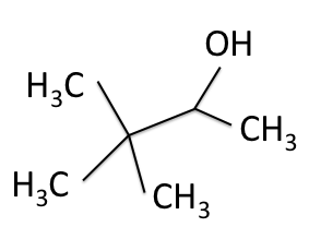
H-NMR Spectrum of 3,3-dimethyl-2-butanol

Each peak in a ^{1}H-NMR spectrum represents a certain number of hydrogen nuclei and describes their neighborhood in the molecule.

^{13} 
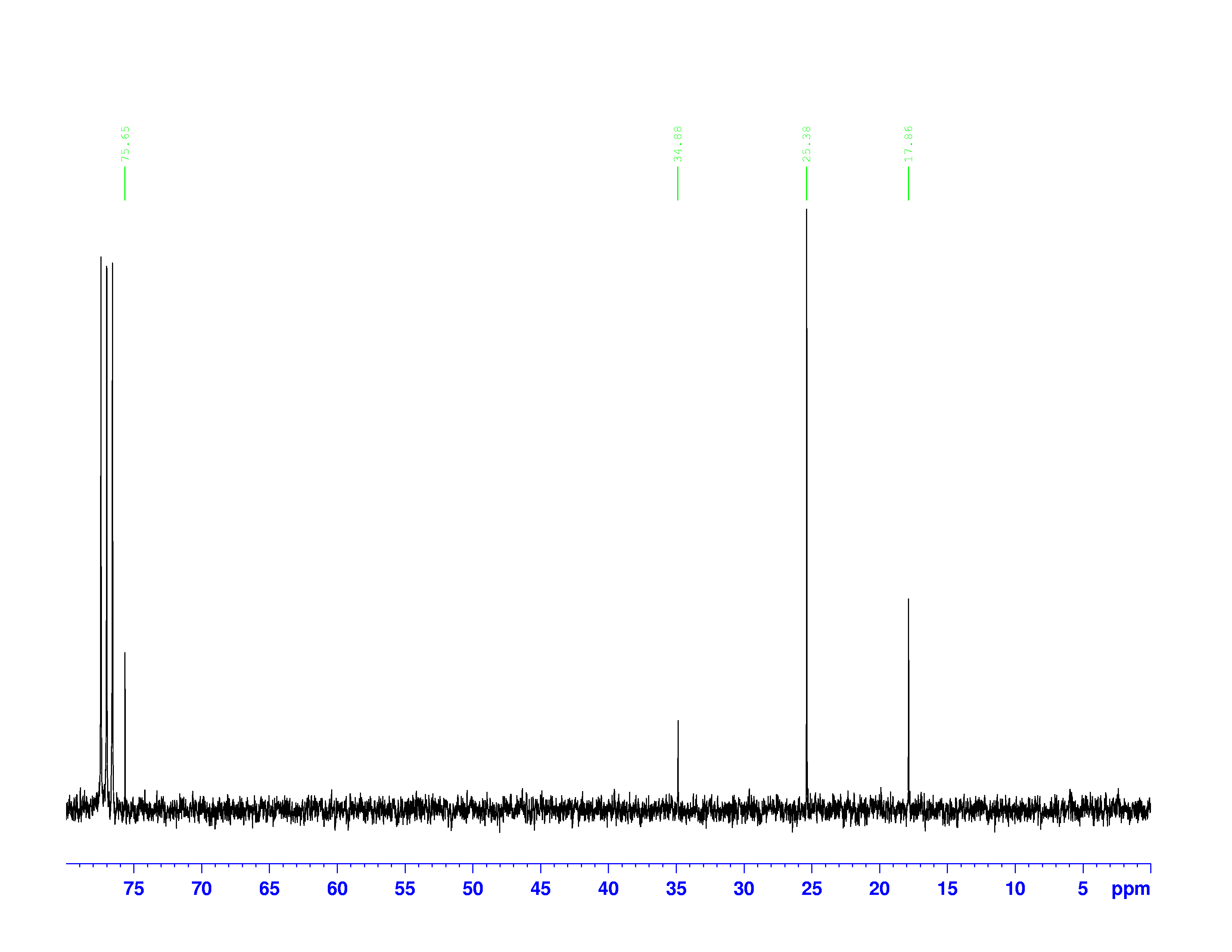
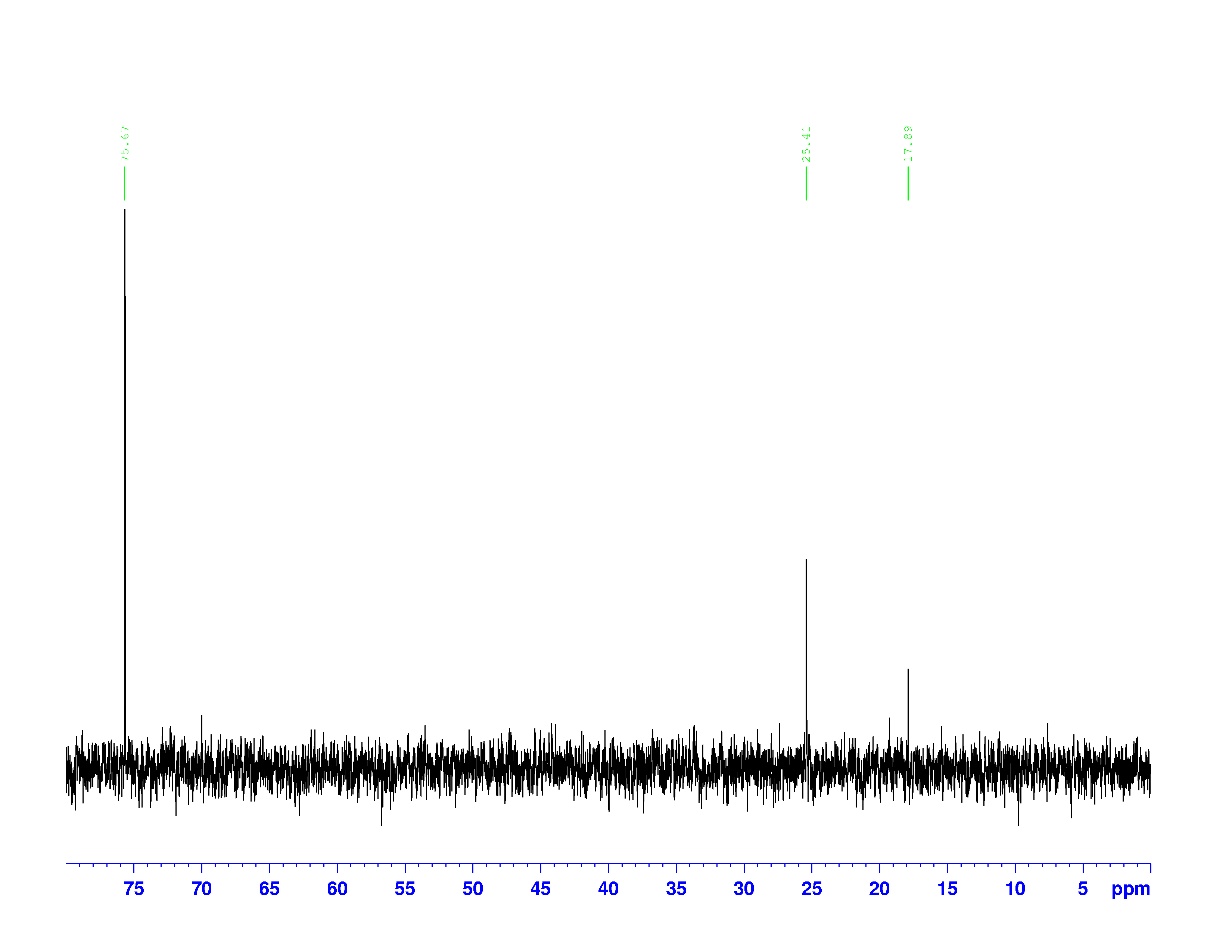
C-NMR spectrum of 3,3-dimethyl-2-butanol

Each peak in a ^{13} C-NMR spectrum represents a specific “type” of carbon in the molecule.  One peak can represent more than one carbon nucleus if they have the same electron densities.

The two spectra below are meant to be read together.

Top:  DEPT-135 Spectrum; Bottom:  DEPT-90 Spectrum

The peaks on these spectra describe the number of hydrogen atoms bound to each carbon atom.  The frequencies of the peaks are the same as they are on the ^{13}C-NMR.

More information on exactly how to interpret each spectrum, and translate all of their information into a molecular structure, is forthcoming.


Share

Polarization Modulation

The modulation of the polarization of a laser to me is the most interesting and applicable use of an EoM. I recall from before this equation

(1)   \begin{equation*} V_{HW}=\frac{\lambda}{2r{n_{0}}^{3}} \end{equation*}

This is the first key modulating the polarization this means once you give it the correct voltage to your EoM it acts like a half wave plate. A half wave plate is an optical element that that allows you to rotate your electromagnetic wave. The corresponding Jones matrix to this is \begin{bmatrix} cos2\theta & sin2\theta\\ sin2\theta&-cos2\theta \end{bmatrix} 
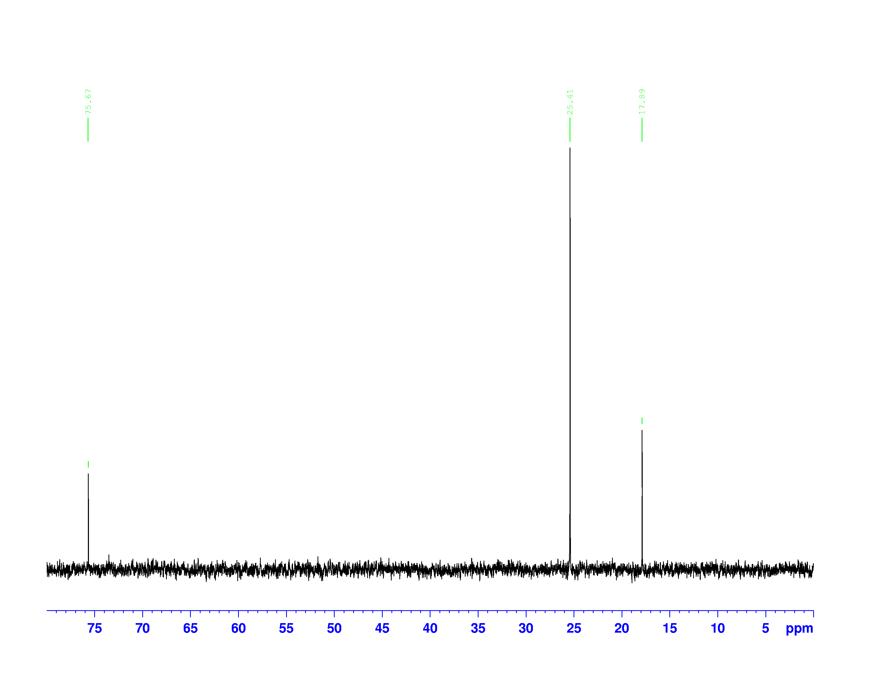
. I will go a little more in depth on different angles effects later on

Okay so before the laser enters the EoM it must be either horizontally or vertically polarized using some kind of polarizer. For example the use of the beam splitter in the figure below

Let’s use the horizontally polarized beam to be the one to go into the EoM so the Jones vector is \begin{bmatrix} E_{x}} \\ 0  \end{bmatrix} and lets orient the EoM to \theta =\frac{\pi }{4} making the half wave plate Jones matrix \begin{bmatrix} 0 & 1\\ 1 & 0 \end{bmatrix} so the effect looks like this

\begin{bmatrix} 0 & 1\\ 1 & 0 \end{bmatrix}\begin{bmatrix} E_x \\ 0 \end{bmatrix}=\begin{bmatrix} 0 \\ E_x  \end{bmatrix}

Notice the E_x is now in the y direction making the laser beam vertically polarized

Lets look at how a half wave plate acts for different \theta. Below is a graph of the amount of E_x, the blue line and the amount of E_y, the red line that will exit the half wave plate as a function of \theta

As you can see that when \theta=\frac{\pi}{4} you have only E_y a predicted above. From this graph you can also see that when \theta=\frac{3\pi}{4} you have equal amounts E_x and E_y

Here is an animation of How the electric field direction will change with different \theta

Mathmatica was giving me a lot of trouble to do this simple task. This still shows how there exists a \theta that will make the electric field switch directions

Share

Phase Modulation

Phase modulation is not a very difficult concept to grasp. In my blog proposal I presented this equation

(1)   \begin{equation*} \frac{1}{n^{2}}=\frac{1}{{n_{0}}^{2}}}+rE+RE^2 \end{equation*}

This allows you to change the index of refraction with an applied electric field. The speed a wave travels inside a new medium is equal to the speed of light in a vacuum divided by the index of refraction of the material v=\frac{c}{n}. Using this relationship and the equation above, we have an expression that relates the applied electric field strength to the speed of the wave in inside the crystal.

(2)   \begin{equation*} {v^{2}}=\frac{c^{2}}{{n_{0}}^{2}}}+rEc^2+RE^2{c^2} \end{equation*}

Once the wave exits the EoM it will have a shift in phase. Being able to vary the speed of the laser inside the crystal very slightly will give you the ability to modulate the phase of the laser so that you can have it exit the EoM at what ever point in its oscillation you wish.

Here is an animation showing a light wave entering a crystal and slowing down having its phase shifted. I could not figure out how to draw lines on the graph but the crystal is from 0 to 2\pi

.

Share

Jones Vectors and Matrices

I think it is important to have an introduction into Jones vectors and matrices. A Jones vector is when you represent the Electric field as such

(1)   \begin{equation*} \vec{E}}=\begin{bmatrix} E_{x}\\E_{y} \end{bmatrix} \end{equation*}

A Jones matrix is a 2 by 2 matrix that does some kind of operation on the Jones vector thereby transforming it. These Jones matrices vary depending on the optical element that your electromagnetic wave is traveling through. Some examples of Jones matrices

Horizontal Polarizer:

\begin{vmatrix} 1 & 0\\ 0& 0 \end{vmatrix}\rightarrow \begin{bmatrix} 1 & 0\\ 0& 0 \end{bmatrix}\begin{bmatrix} E_{x}\\ E_{y}  \end{bmatrix}=\begin{bmatrix} E_{x}\\ 0  \end{bmatrix}

Vertical Polorizer:

\begin{vmatrix} 0 & 0\\ 0& 1 \end{vmatrix}\rightarrow \begin{bmatrix} 0 & 0\\ 0& 1 \end{bmatrix}\begin{bmatrix} E_{x}\\ E_{y}  \end{bmatrix}=\begin{bmatrix} 0\\E_{y} \end{bmatrix}

Half wave plate:

\begin{vmatrix} cos2\theta & sin2\theta\\ sin2\theta& -cos2\theta \end{vmatrix}\rightarrow \begin{bmatrix} cos2\theta & sin2\theta\\ sin2\theta& -cos2\theta \end{bmatrix}\begin{bmatrix} E_{x}\\ E_{y}  \end{bmatrix}=\begin{bmatrix} E_{x}cos2\theta+E_{y}sin2\theta\\E_{x}sin2\theta-E_{y}cos2\theta  \end{bmatrix}

\theta is the angle that the half wave plate is oriented at. These Jones vectors will be useful in describing how the electromagnetic wave is polarized in the following posts

Share