
The equations and plots I present here all consider a positive point charge with constant velocity v starting at the origin at time t = 0, and moving along the z axis. They derive from Griffiths example 10.3.
First we take the simplest case. If we consider the electric potential at the origin (r = 0) over time as the particle moves upward, we have:
(1) 
Note that the potential does not depend on the speed of light. This is due solely to the fact that the particle begins moving from the same point we are considering; the speed of light is only of import when at t = 0 there is some electromagnetic information which has not yet reached the point we are considering, for then we need to know how fast that information is traveling.
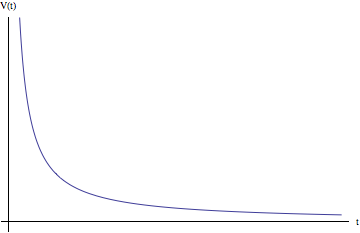
The above is a familiar graph where V is proportional to the reciprocal of t. As we can see, the origin’s potential is infinite as time t = 0 (because the point charge is located there), and as the charge moves away along the z axis the potential falls off to zero asymptotically.
The next equation modifies Griffiths 10.42. We express the dot product in the denominator using cosine, expressing the desired angle in terms of x, y and z.
(2) ![\begin{equation*} V = \frac{qc}{\sqrt{\left(c^2t-\frac{vz\sqrt{x^2+y^2+z^2}}{x^2+y^2+z^2}\right)^2 +\left(c^2-v^2\right)\left(x^2+y^2+z^2-c^2t^2\right)\right]}} \end{equation*}](https://pages.vassar.edu/magnes/wp-content/ql-cache/quicklatex.com-bb03d4a473db4f0166ae6687bb56e5f7_l3.png "Rendered by QuickLaTeX.com")
The original Mathematica code for the following animations allows many different values of z and t, but I’ve posted two possible configurations below. The first is where z is positive, so the charge passes us at some point (hence the potential grows larger at first), and the second is the special case where z is zero, which describes the potential of the xy plane over time.
http://www.youtube.com/watch?v=oZV94lqzmeE http://www.youtube.com/watch?v=rt9h4XljEnE&feature=channel&list=ULNote: in the first animation there is an asymmetry in the electric potential near the origin that becomes evident at times where the potential grows large. However, the x and y variables in 10.42 are completely interchangeable, and I am unable to come up with a physical or mathematical argument for this. It may indicate a problem with Mathematica’s sampling rate near large function outputs.
Similar to the graph above the potential in both animations decreases very quickly at first, then more slowly. We can write the denominator of Griffiths 10.42 as a polynomial in t:
(3) 
Since polynomials are dominated by their leading term for large values, the denominator of 10.42 is approximately t for large values of t. Thus for large values of t, the electric potential decreases in a way similar to the origin case (where V is proportional to the reciprocal of t), but in general will decrease faster. Considering the origin is a subcase of considering the entire xy-plane; this means it represents a special sort of minimum: one where the electric potential will fall off more slowly than anywhere else! This makes sense in terms of the physical situation: at any time, the point in the xy-plane closest to the point charge is the origin. The surprising part is how much that makes a difference. Whereas for the origin case the electric potential decreases proportional to the 1/t, for the rest of the xy plane it decreases proportional to 1/t^2.
The magnetic vector potential due to a point charge with constant velocity should also go to zero for large values of t, but I’m having trouble getting my current models to reflect this. Vector models and animations for this are to come, as well as for the event horizon problem presented as 10.15 in Griffiths.
