Category Archives: Christian

Project Results

Using Griffiths Example 10.3 as a roadmap, I’ve attempted to derive an equation describing the electric potential due to a point charge moving in uniform circular motion. My complete derivation (available here) is too long to post in its entirety, but I’ve outlined it below. It relies heavily on vector algebra, and on a few equations from Griffiths.

First I express a uniform circular trajectory in spherical coordinates:


(1)   \begin{equation*}    \vec{W}(t)=R\hat{r}-\frac{\pi}{2}\hat{\theta}-wt_r\hat{\phi}    \end{equation*}

Then I use Griffiths 10.33 to find an expression for the retarded time. This requires solving the quadratic function in $t_r$, and then making a few clever comparisons (see the full proof) to obtain the correct solution sign. In the end it comes out to be:

(2)   \begin{equation*}       t_r=\frac{ (tc^2-w\phi) - \sqrt{(w\phi+tc^2)^2-\clubsuit(c^2t^2-(r-R)^2+\pi\theta-(\theta')^2}}{\clubsuit}          \end{equation*}

Where I’ve let the $\clubsuit = (c^2-w^2)$ in order to have the equation fit on the page.

I then use Griffiths 10.33 and 10.34 to obtain expressions for the script r vector. In particular, I find a useful expression for the denominator of the Liénard-Wiechert electric potential:

(3)   \begin{equation*}     \scripty{r}c-\vec{\scripty{r}} \cdot \vec{v} = c^2t-\phi wR-(c^2+Rw)t_r     \end{equation*}

Where $t_r$ is defined by equation (2) above. This allows for a substitution directly into the Liénard-Wiechert potential equation (Griffiths 10.39):

(4)   \begin{equation*}        V(\vec{r},t)=\frac{1}{4\pi \varepsilon_0} \frac{qc}{(c^2t-\phi wR-(c^2+Rw^2)t_r})   \end{equation*}

Here I’ve refrained from substituting in for $t_r$ in the interest of space. I’ve created some Mathematica code to plot this derived expression for the electric potential, but I had difficulties exporting it. A quick look at the code reveals why: there are two large regions where the value of the potential is indeterminate. I’m unable to come up with a physical explanation for this, but a mathematical one follows quickly from a look at the denominator of the potential function. Essentially the problem is there exist values of $r$, $\phi$, and $t$ that allows the radicand to become negative, which results in a complex value for the potential. Taking the absolute value does eliminate this problem, but the physical motivation for making such a move is unclear.

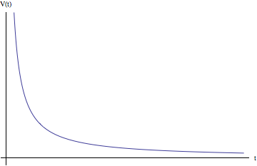
As far as the function itself goes, it makes me wonder if there’s not some mistake in my derivation. There are aspects of the physical situation that I feel it models well: the spiral shape, the smoothness near points of maximum potential; for a idea of why the spiral shape is accurate, check out this article, particularly Figure 1 (J.H Hannay, M.R Jeffrey). But the problems are glaring. For one thing, the function isn’t periodic- it drops off to zero for large values of t. Our particle is moving in uniform circular motion, so the resulting potential should reflect that by oscillating as well. The indeterminate regions I mentioned above are also a problem – the electric potential should be defined all regions of the coordinate system. The other issue is that the arms of the spiral cease abruptly after a certain radius- there should be a gradual decrease in potential for larger and larger values of r.

I was able to fix a Mathematica problem that I mentioned in the Preliminary section. One of my animations was exhibiting a suspicious asymmetry, which I discovered was due to an idiosyncrasy of Mathematica’s evaluation. The fixed video is below. It represents the potential due to a point that begins at rest at the origin and moves along the $z$ axis with constant velocity.

Share

Conclusion

Overall I’m happy with my models and analysis for the non-accelerating point charge. The Mathematica animations demonstrate that the equations describe their physical counterparts well, and the proportionality between the electric potential and time for different spacial assumptions was interesting to investigate. Ideally I would have been able to adequately represent the magnetic vector potential field in Mathematica as well.

With more time I’d also try to generate a better model for the circular motion case, whether that means finding a mistake in my derivation or using a different underlying assumption or driving equation. I’d be interested in investigating other particle trajectories as well, perhaps defining more intricate ones but imposing a time-domain restriction.

And of course, there’s always the electric and magnetic fields themselves. To derive the E and B fields for a few simple particle trajectories would be interesting and challenging, and might segway well into some of the material from Griffiths relativity chapter. On page 528 is an alternate derivation for equation 10.68, which is the electric field of a moving point charge. The chapter 12 derivation is described as being both more efficient and more intuitive, and I think it would be worthwhile to take the time to compare the two. Problem 10.15 presents another relativity topic I would have liked to reach: the event horizon. The concept of retarded time is closely linked to any explanation of time dilation or simultaneity,  and I would try to unfold the problem with this in mind.

Share

Preliminary Results

The equations and plots I present here all consider a positive point charge with constant velocity v starting at the origin at time t = 0, and moving along the z axis. They derive from Griffiths example 10.3.

First we take the simplest case. If we consider the electric potential at the origin (r = 0) over time as the particle moves upward, we have:

(1)   \begin{equation*} V(t) = \frac{qc}{\sqrt{(c^2t)^2+(c^2-v^2)(-c^2t^2)}} =\frac{q}{vt} \end{equation*}

Note that the potential does not depend on the speed of light. This is due solely to the fact that the particle begins moving from the same point we are considering; the speed of light is only of import when at t = 0 there is some electromagnetic information which has not yet reached the point we are considering, for then we need to know how fast that information is traveling.

The above is a familiar graph where V is proportional to the reciprocal of t. As we can see, the origin’s potential is infinite as time t = 0 (because the point charge is located there), and as the charge moves away along the z axis the potential falls off to zero asymptotically.

The next equation modifies Griffiths 10.42. We express the dot product in the denominator using cosine, expressing the desired angle in terms of x, y and z.

(2)   \begin{equation*} V = \frac{qc}{\sqrt{\left(c^2t-\frac{vz\sqrt{x^2+y^2+z^2}}{x^2+y^2+z^2}\right)^2  +\left(c^2-v^2\right)\left(x^2+y^2+z^2-c^2t^2\right)\right]}}          \end{equation*}

The original Mathematica code for the following animations allows many different values of z and t, but I’ve posted two possible configurations below. The first is where z is positive, so the charge passes us at some point (hence the potential grows larger at first), and the second is the special case where z is zero, which describes the potential of the xy plane over time.

Note: in the first animation there is an asymmetry in the electric potential near the origin that becomes evident at times where the potential grows large. However, the x and y variables in 10.42 are completely interchangeable, and I am unable to come up with a physical or mathematical argument for this. It may indicate a problem with Mathematica’s sampling rate near large function outputs.

Similar to the graph above the potential in both animations decreases very quickly at first, then more slowly. We can write the denominator of Griffiths 10.42 as a polynomial in t:

(3)   \begin{equation*}           \sqrt{ (v^2 c^2)t^2- (2c^2\vec{r} \cdot \vec{v})t + c^2r^2 -v^2r^2+( \vec{r} \cdot \vec{v})^2           \end{equation*}

Since polynomials are dominated by their leading term for large values, the denominator of 10.42 is approximately t for large values of t. Thus for large values of t, the electric potential decreases in a way similar to the origin case (where V is proportional to the reciprocal of t), but in general will decrease faster. Considering the origin is a subcase of considering the entire xy-plane; this means it represents a special sort of minimum: one where the electric potential will fall off more slowly than anywhere else! This makes sense in terms of the physical situation: at any time, the point in the xy-plane closest to the point charge is the origin. The surprising part is how much that makes a difference. Whereas for the origin case the electric potential decreases proportional to the 1/t, for the rest of the xy plane  it decreases proportional to 1/t^2.

The magnetic vector potential due to a point charge with constant velocity should also go to zero for large values of t, but I’m having trouble getting my current models to reflect this. Vector models and animations for this are to come, as well as for the event horizon problem presented as 10.15 in Griffiths.

Share

Time Dependent Potentials and Fields – Proposal

My project will be based on the theoretical content of Chapter 10 of Griffiths, which deals with the previous equations for the electric and magnetic potentials (and fields) of charges, but with the additional dimension of time. My goal is not to rewrite Griffiths’ chapter, but rather to gain a deeper understanding of the equations he presents through graphical analysis. Central to the difference between the old equations and the new time-dependent ones is the concept of retarded time, which is defined as

(1)   \begin{equation*} t_r \equiv t - \frac{|\vec{r} - \vec{r}\ '|}{c} \end{equation*}


(David J. Griffiths, Introduction to Electrodynamics)

Where t is the actual time, the r vector represents the position of a given point in the system, the r’ vector represents the position of the charge, and c is the speed of light a vacuum. The second term represents a delay- how long it takes for the electromagnetic information to travel from the charge to a given point in space. Thus retarded time embodies the idea that electromagnetic messages take time to propagate through space, and in fact propagate at the speed of light. This means that the present position of a particle becomes incidental. At any given time there exists an effective position, illustrated below:


For a more in depth discussion of effective position (in three dimensions), see page 430 of Griffiths. In any case, our definition of retarded time leads to a time-dependent generalization of the potential equations:

(2)   \begin{equation*} V(\vec{r},t) = \frac{1}{4 \pi \varepsilon_0} \int \frac{\rho(\vec{r}\ ',t_r)}{|\vec{r}-\vec{r}\ '|}d \tau' \end{equation*}


(3)   \begin{equation*} \vec{A}(\vec{r}, t) = \frac{\mu_0}{4 \pi} \int \frac{\vec{J}(\vec{r} \ ', t_r)}{|\vec{r} - \vec{r} \ ' |} d \tau' \end{equation*}


(David J. Griffiths, Introduction to Electrodynamics)

Which are nearly identical to previous definitions of the potentials, with the exception that both the charge density and the current density now depend on the retarded time. These potentials can be used to derive Jefimenko’s Equations, which describe the non-static electric and magnetic fields of an arbitrary continuous charge distribution. I have omitted them here; since they rely so heavily on vector notation, at this point I’m unsure whether Mathematica’s plotting capabilities will be useful in obtaining graphical representations of them or the above potentials. I intend to explore manipulating them into a form easier to graph, or perhaps examine them in the plane z = 0. Additionally, choosing a simplistic charge distribution may result in an expression that could be graphed more readily.

In any case, I want to focus more on the electrodynamics of moving point charges. Their potentials, which can be expressed without an integral, are referred to as the Liénard-Wiechert Potentials:

(4)   \begin{equation*} (i)\ \ V(\vec{r}, t) = \frac{1}{4\pi \varepsilon_0} \frac{q c}{\vec{v}(c|\vec{r} - \vec{r} \ '| -(\vec{r} - \vec{r} \ ')} \ ,\  (ii) \ \  A(\vec{r}, t) = \frac{\vec{v}}{c^2}V(\vec{r},t) \end{equation*}

(David J. Griffiths, Introduction to Electrodynamics)

I believe these equations will prove easier manipulate and graph, and may apply restrictions such as the assumption that the dot product in the denominator is zero. Additionally I’ll examine these equations in only two spacial dimensions (various vertical and horizontal planes).

The following equation can be derived from Jefimenko’s (see Griffiths’ Example 10.3), but I have made a few assumptions of my own: that the velocity is constant and that the position vector r is perpendicular to the velocity vector v. Additionally, I’ve expressed the position r in terms of x and y, and let z = 0.

(5)   \begin{equation*} V(x,y,t) = \frac{q c}{\sqrt{(c^2t)^2+(c^2-v^2)(x^2+y^2-c^2t)}} \end{equation*}


Using Mathematica and plugging in a few values, I was able to generate a preliminary animation:

This is the kind of result I’d like to obtain for a number of other cases, magnetic as well as electric. I think it will be easy to formulate constraints for linear and quadratic charge accelerations, as well as circular motion, and applying them to the Liénard-Wiechert Potentials will hopefully yield workable results. Ideally I’ll have a number of equations and animations and be able to select and pursue the most interesting for presentation.

Share

Blog Proposal

Electrodynamics is concerned with answering a simple question: what is the force exerted on a test charge Q by some arbitrary configuration of charge? Griffiths does not achieve the equation that truly answers this until the tenth chapter; while powerful, the relationship is complex. My goal is to explore this overarching equation and the ideas directly preceding it, including the Liénard-Wiechert Potentials, Jefimenko’s Equations, and retarded time. In order to deal with the five dimensional nature of these equations I will make heavy use of Mathematica’s plotting and manipulation functions. My hope is to generate a number of graphical representations of these functions, some with simplifying assumptions made, and thereby expose their physical significance.

Share