In Vassar’s 300 MHz NMR, the Larmor frequency of an unaltered hydrogen nucleus with shielding factor  is 300 MHz.
  C nuclei are different than
  H nuclei, and have a different Larmor frequency in the spectrometer’s 7.046
  magnetic field. According to Jacobsen in “NMR Spectroscopy Explained,” the Larmor frequency of unaltered C nuclei with is 75.43 MHz in this magnetic field. The magnetogyric ratio
  , is 672.650
 We bring back the equation for Larmor Frequency:
(1) 
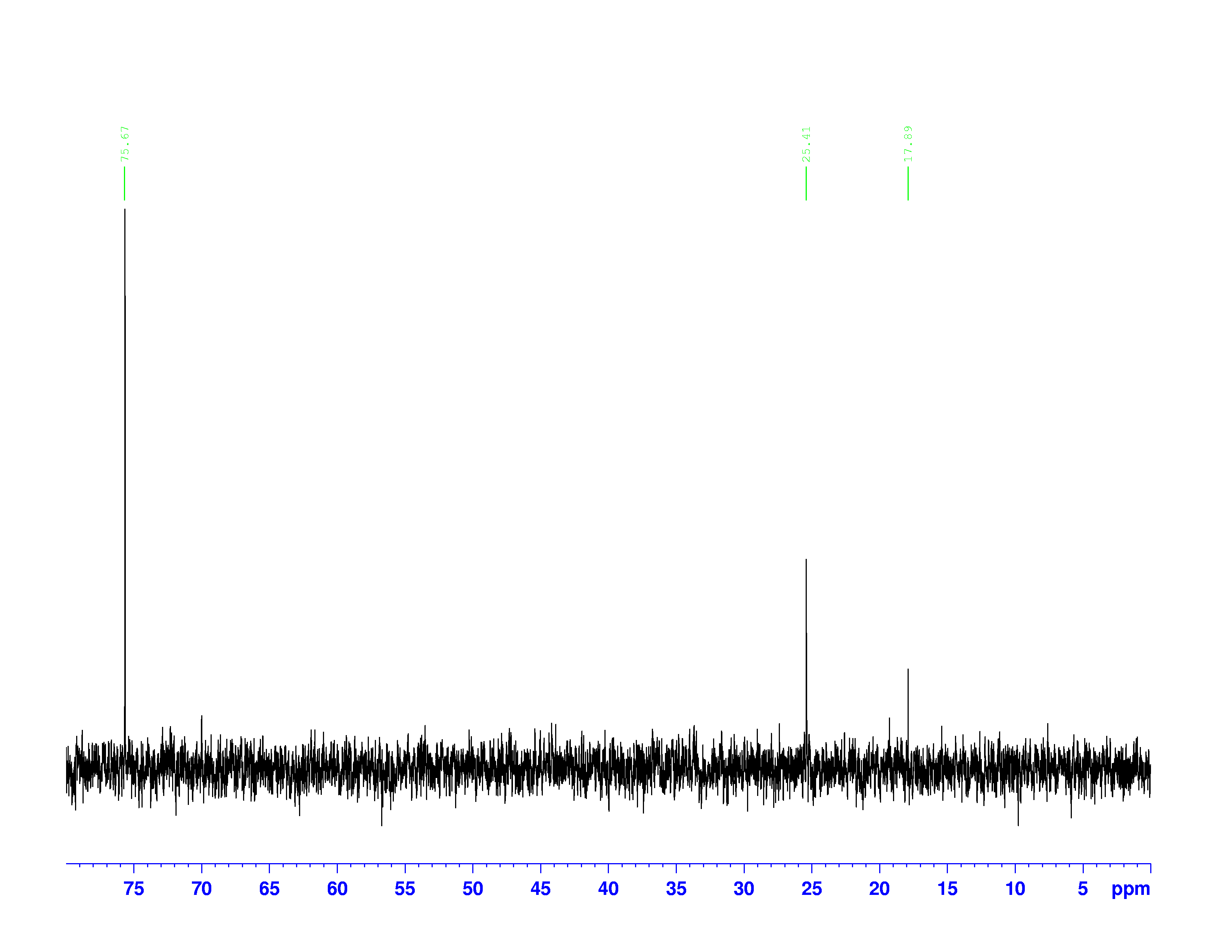
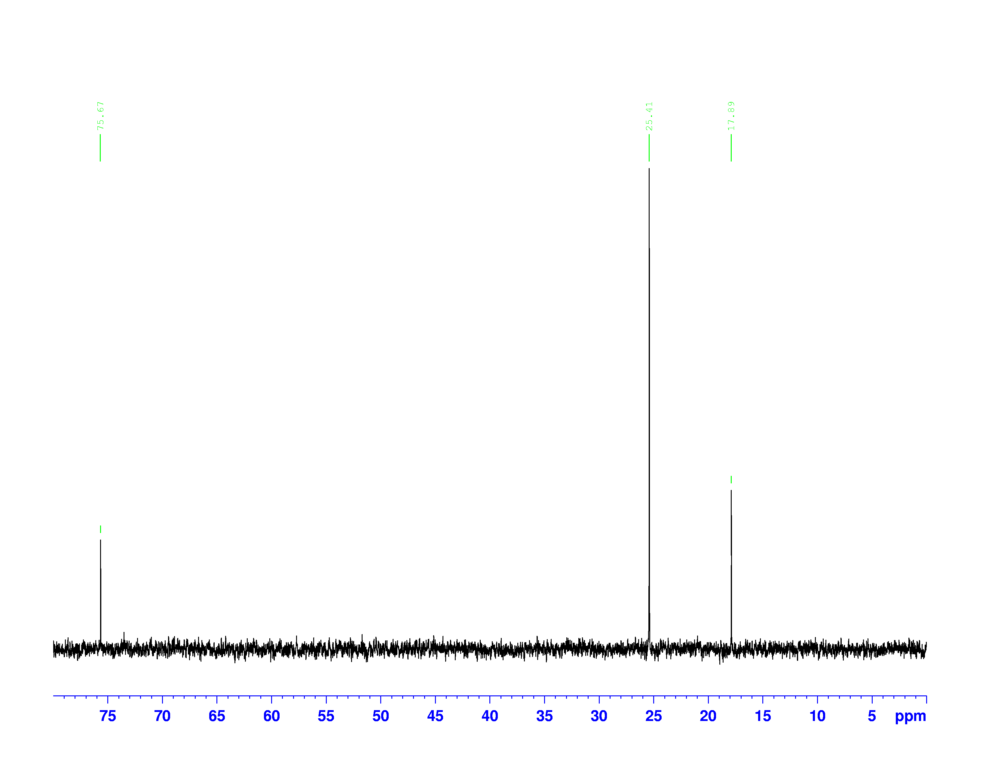
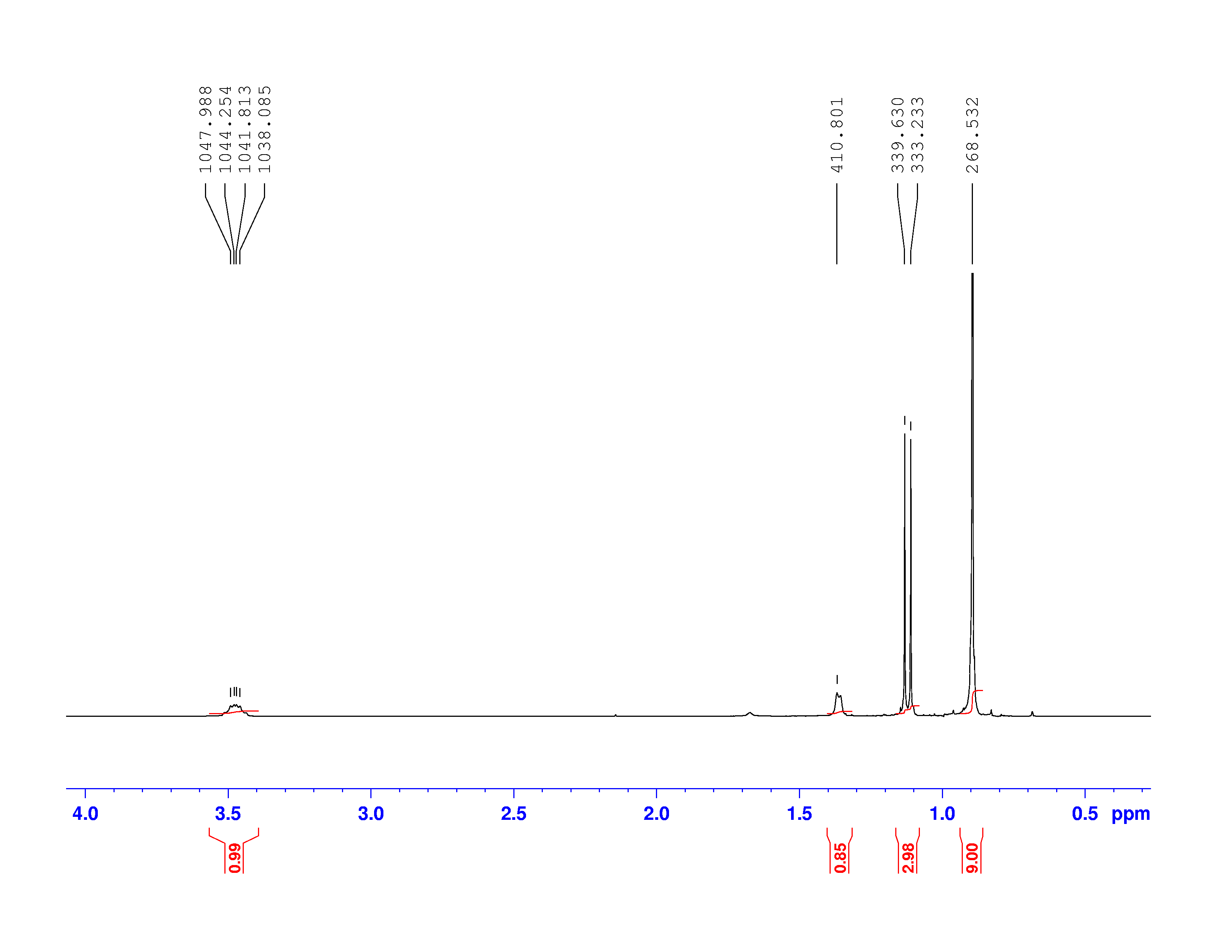
You might ask why C nuclei are the focus of carbon NMR instead of the much more common and ordinary  C nuclei. It comes down to the composition of the nucleus. Only nuclei with nonzero spin are magnetically active. Spin is a type of angular momentum intrinsic to subatomic particles. Particles with nonzero spin can have magnetic moments that can be influenced by a magnetic field. Any nucleus with an even number of protons and an even number of neutrons will not be magnetically active because its spin is 0 and it has no magnetic moment. Carbon-12 has 6 protons and 6 neutrons, so it can’t be studied with NMR. Carbon-13 has 6 protons and 7 neutrons, so we can study it with NMR. The structure and C-NMR spectrum of 3,3-dimethyl-2-butanol is shown below.

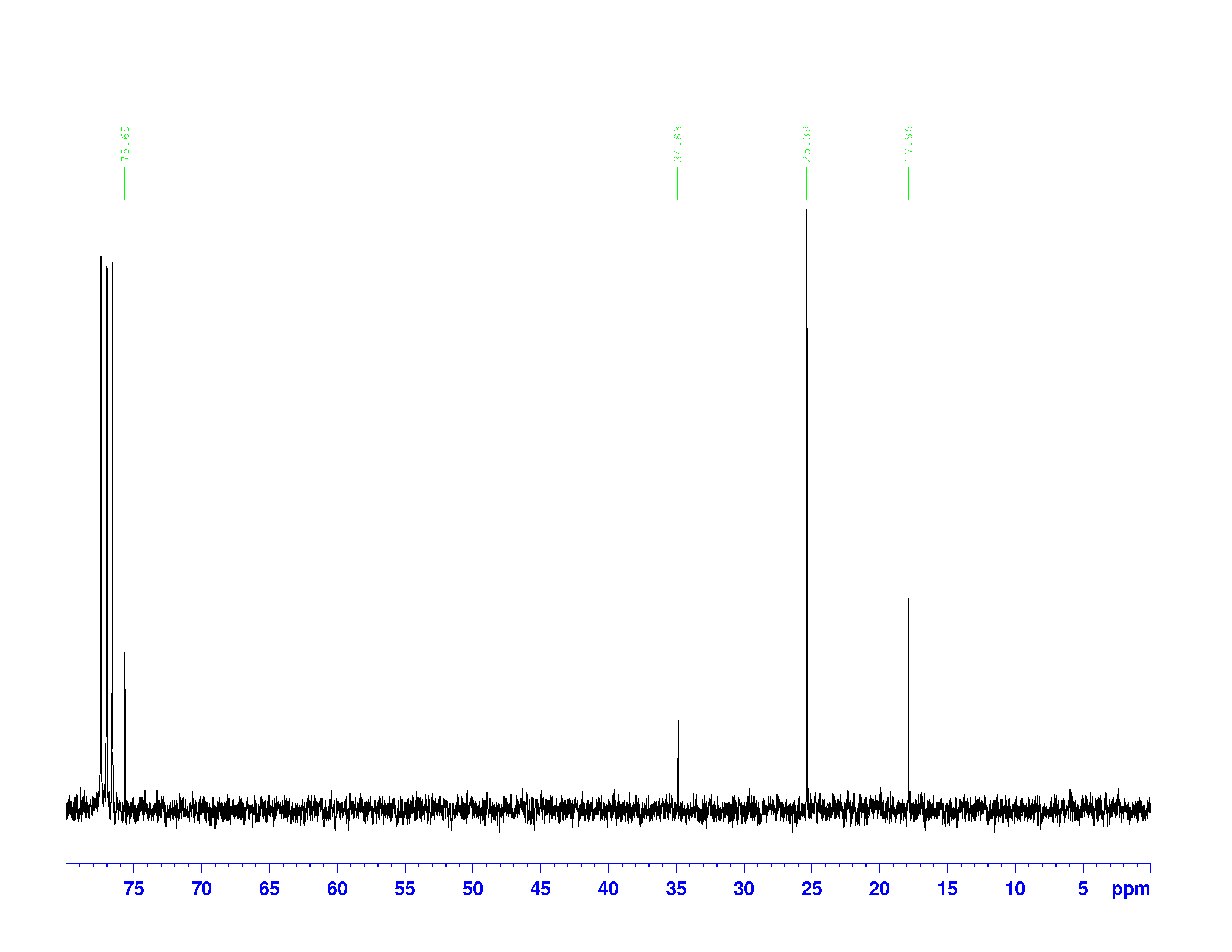
At first glance, the spectrum looks almost the same as the H-NMR spectrum. However, there is little indication of how many carbons a single peak is referring to. Each peak corresponds to a type of carbon in the molecule. The triplet peak at 77 ppm represents the deuterated chloroform, CDCl , used to dissolve the sample. Excluding that triplet, the molecule has four different kinds of carbon. To help us find what carbons are represented here, we turn to the other two spectra of interest. They are called the DEPT-90, and the DEPT 135. DEPT stands for Distortionless Enhancement by Polarization Transfer. The technique hits the sample with five successive radio pulses designed to excite either hydrogen or C nuclei. The sequence of pulses is:
- A hydrogen pulse at 90° from the x-axis
- A hydrogen pulse at 180° from the x-axis plus a carbon pulse at 90° from the x-axis.
- A carbon pulse at 180° from the y-axis plus a hydrogen pulse at either 45°, 90°, or 135° from the y-axis.
The angle of the last hydrogen pulse is the number in the DEPT label. DEPT-90 ends with a hydrogen pulse at 90° from the y-axis. The pulse sequence is modeled below for DEPT-90 as an example. Red waves are hydrogen pulses, green waves are carbon pulses:
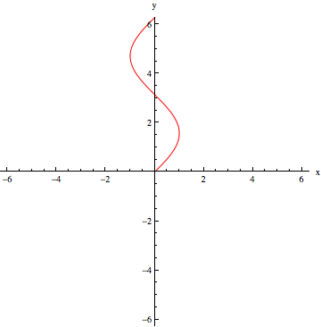
DEPT-90 Pulse 1
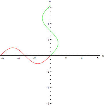
DEPT-90 Pulse 2
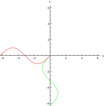
DEPT-90 Pulse 3
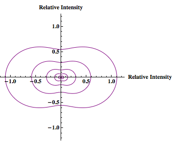
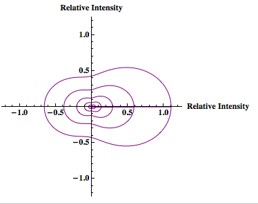
These combinations of pulses result in transfers of polarization between the hydrogen and carbon nuclei. Different combinations pick out carbons with one, two, or three hydrogens attached to them. The DEPT-90 and DEPT-135 spectra are shown below:
 DEPT-90 spectrum
 DEPT-135 Spectrum
The chemical shifts of the peaks on these two spectra are the same as they are on the C-NMR spectrum. The sizes of the peaks on the two spectra are different, and this size difference is the key to understanding them. You may have noticed the peak at 35 ppm on the C-NMR spectrum doesn’t appear on either of the DEPT spectra. This is because DEPT spectra only show carbons with hydrogens attached to them. Therefore the 35 ppm peak represents the carbon in 3,3-dimethyl-2-butanol with no hydrogens on it.
The three peaks on the DEPT spectra are distinguished by their relative directions and sizes on each spectrum.
- Peaks that point up on the DEPT-135, point up on the DEPT-90, and are larger on the DEPT-90, represent carbons with one hydrogen attached.
- Peaks that point down on the DEPT-135 represent carbons with two hydrogens attached.
- Peaks that point up on the DEPT-135, point up on the DEPT-90, and are smaller on the DEPT-90 represent carbons with three hydrogens attached.
- Carbons without hydrogens don’t appear on either the DEPT-135 or DEPT-90
These are not the most general rules for interpreting DEPT-90 and DEPT-135 spectra. Normally, carbons with two and three hydrogens don’t appear on the DEPT-90 spectra. However, in this experiment the radio pulse used to collect the data was too long. This causes the DEPT-90 spectrum to contain a small fraction of the DEPT-135 spectrum’s information.
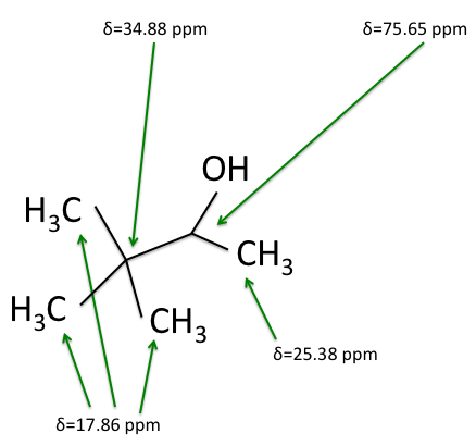
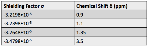
Armed with this new information from the DEPT spectra, we can determine which carbons are represented by which peaks on the C-NMR spectrum, and calculate their shielding factors. A table of chemical shift and shielding factor values for each C nucleus in 3,3-dimethyl-2-butanol is below.

The same trend that applies to hydrogen nuclei applies to C nuclei. The more negative the shielding constant, the lower the electron density around the nucleus, and the higher the effective magnetic field felt by the nucleus. C nuclei also experience higher chemical shifts compared to hydrogen nuclei because they are bonded to more atoms and have more opportunity to be deshielded when those atoms take electron density.
The figures below shows the structure of 3,3-dimethyl-2-butanol with the carbons labeled with their corresponding chemical shifts. This is the final step in reconstructing the molecule from the NMR data.


![\begin{equation*} \frac{\partial^2}{\partial z^{2}}\widetilde{E}_{2}= \frac{\partial}{\partial z} [ \frac{\partial A_{2}}{\partial z}e^{i(k_{2}z-wt)} +ik_{2}A_{2}e^{i(k_{2}z-wt)}] \end{equation*}](https://pages.vassar.edu/magnes/wp-content/ql-cache/quicklatex.com-7346f50874aa7a9ddf5dfa433a9dd721_l3.png "Rendered by QuickLaTeX.com")
![\begin{equation*} \frac{\partial^2}{\partial z^{2}}\widetilde{E}_{2}= [ \frac{\partial^{2} A_{2}}{\partial z^{2}} +ik_{2}\frac{\partial A_{2}}{\partial z}+ ik_{2} \frac{\partial A_{2}}{\partial z} -k^{2}_{2}A_{2}]e^{i(k_{2}z-wt)} \end{equation*}](https://pages.vassar.edu/magnes/wp-content/ql-cache/quicklatex.com-7b620256237c766c7ee7484b9782369e_l3.png "Rendered by QuickLaTeX.com")
![\begin{equation*} -[ \frac{\partial^{2} A_{2}}{\partial z^{2}} + 2ik_{2} \frac{\partial A_{2}}{\partial z}-k^{2}_{2}A_{2}]e^{i(k_{2}z-wt)} -\frac{\omega^{2}_{2}}{c^{2}}\epsilon^{(1)}(\omega_{2})A_{2}e^{i(k_{2}z-wt)} =\frac{4\pi \omega^{2}_{n}}{c^2}\bullet2dA^{2}_{1}e^{i(2k_{1}z-\omega_{2}t)} \end{equation*}](https://pages.vassar.edu/magnes/wp-content/ql-cache/quicklatex.com-24c96f68b7ced19254b132c2e1fd5380_l3.png "Rendered by QuickLaTeX.com")
![\begin{equation*} -[ \frac{\partial^{2} A_{2}}{\partial z^{2}} + 2ik_{2} \frac{\partial A_{2}}{\partial z}-k^{2}_{2}A_{2} -\frac{\omega^{2}_{2}}{c^{2}}\epsilon^{(1)}(\omega_{2})A_{2}]e^{i(k_{2}z-wt)} =\frac{8\pi \omega^{2}_{2}}{c^2}dA^{2}_{1}e^{i(2k_{1}z-\omega_{2}t)} \end{equation*}](https://pages.vassar.edu/magnes/wp-content/ql-cache/quicklatex.com-83a3b5e79ed5319e3db777f34f5ff1b2_l3.png "Rendered by QuickLaTeX.com")
![\begin{equation*} [ \frac{\partial^{2} A_{2}}{\partial z^{2}} + 2ik_{2} \frac{\partial A_{2}}{\partial z}]e^{i(k_{2}z-wt)} =-\frac{8\pi \omega^{2}_{2}}{c^2}dA^{2}_{1}e^{i(2k_{1}z-\omega_{2}t)} \end{equation*}](https://pages.vassar.edu/magnes/wp-content/ql-cache/quicklatex.com-970db0321d719adf93489f36e27bd686_l3.png "Rendered by QuickLaTeX.com")


 for each nucleus. The shielding factor is another measure of the relative electron density around each nucleus.
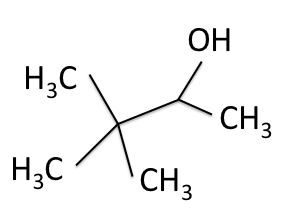
 ) doped with magnesium oxide (MgO). The magnesium oxide is there to prevent optical damage that can occur with high energy light in the bluish green frequencies. The Index of refraction of this crystal is
  = 2.29 and the linear electro optic coefficient r = 30.9. I could not find any information on R the quadratic electro optic coefficient. Inside the EoM, the crystal has a parallel plate capacitor across it as shown below.


 as it passes through the EoM. The yellow wave is resultant amplitude modulation.
 . A quick calculation using:


 , where
  is the number of peaks. The definition of “nearby” is usually 1 carbon atom over in the molecule from the one the original hydrogen is attached to.