
As much as astronomers hate to be mistakenly called astrologers, a little astrological mumbo-jumbo can’t hurt. Astrology is based in the saying “As above, so too below.” This means that there is a relationship between the movements of the planets and what happens on Earth. Because of this, each planet has a purpose or area of life with which it corresponds. Mercury rules all types of communication, including listening, speaking, learning, reading, editing, researching, and negotiating. One of the most well known astrological tropes these days is ‘Mercury in retrograde.’ The terminology here is wrong, Mercury is not ‘in’ retrograde, it is just retrograde. When a planet retrogrades, astrologically it is in a resting or sleeping state, and by extension, the activities it governs do not have their planet to govern them properly. As a result, when Mercury is retrograde, communication tends to break down which can result in some (non-physics-realated) chaos.
With all of that aside, retrograde motion is a bizarre visual phenomenon that puzzled ancient astronomers to no end, especially those who believed in a geocentric model of the solar system. In ancient Greece, the theory of epicyclical motion was formalized. It was used to explain the variations in speed and direction of the five planets known at the time, which I present here. The planets beyond Saturn are too far out and orbit too slowly to present in this project. As it is, it takes around 3 hours to run Saturn for 500π without multiplying the time by a constant.
The geocentric epicycle model proposed that as a planet traveled around Earth in a circular orbit on a path called the deferent, it also traveled in a smaller circular orbit in the same direction, the epicycle, causing the planets orbit to appear like a spiral that backtracked on itself and at times seemed to pause altogether.
Figure 1

The epicycle model was highly accurate because any smooth curve can be approximated to arbitrary accuracy with a sufficient number of epicycles, as would later be shown by Fourier analysis. Retrograde motion was not understood to be an illusion until the 1500s, when Copernicus proposed the heliocentric model. Towards the 1600s, Kepler’s revelations in astronomy further disproved the epicyclic models by proving that the planets orbited in elliptical paths rather than circular. Kepler’s third law states t^2∝ a^3, the period of orbit squared is proportional to the semi-major axis of its orbit.
Figure 2

The figure above illustrates this law. The sun is at one of the foci in the elliptical orbit. When a planet is traveling from a to b, it is near perihelion, the point in the orbit closest to the sun. The planet travels fastest in this area, slingshotting around the sun and covering distance ab at time t1, sweeping out the area a1. When traveling from c to d, the planet is near aphelion, the furthest point in its orbit from the sun, causing it the travel more slowly. At this point, the planet travels distance cd at time t2, sweeping out the area a2. Because of Kepler’s third law, and the varying speeds of the orbit at different point of orbit, t1=t2 and a1=a2.
The planets in the solar system have much lower eccentricities than what I’ve illustrated above. However, Kepler’s law proves that planets with greater semi-major axis have greater periods of orbit, which account for the differential speeds of orbit and by extension the apparent retrograde motion.
Retrograde occurs when an inner planet laps and passes and outer planet. From the inner planet’s perspective, the outer planet appears to slow in the sky and then reverse its orbit for a time, before continuing forward again.
Figure 3

The result is a loop or zig-zag in the sky over time.
Figure 4

For my project, I wanted to create a simulation that would plot the retrograde motion in the sky in a way that looked like Figure 3, showing the planets orbiting and showing a line of sight plotting out the typical retrograde loop. I ended up with something different.
The purpose of my project is educational, to illustrate a concept which is difficult to grasp when witnessing it in nature and greatly benefits from additional visual aids. By plotting the orbits and retrogrades simultaneously, the relationship between the positions of the planets and the observed retrograde motion becomes more clear.
I decided to ignore Kepler’s elliptical orbits, in favor of a simpler circular orbit, which is easier to plot in Matlab. The eccentricity of the planets in our solar system is very low, with Mercury and Pluto having the greatest eccentricities of just over .2 each, so the error caused by this exception is relatively low. I also ignored the effects of gravity between planets because this force does not affect apparent retrograde motion noticeable. I plotted only two planets at a time – Earth and whichever planets retrograde would be simulated.
Using each planets semi-major axis and orbital period, I calculated the number of degrees which each planet travels in a day to simulate the relative speeds of the planets.
Figure 5

Once the planets were orbiting properly, I decided to plot the relative X and Y positions of the planets versus time. The longer the two planets orbited, the more obvious a pattern of sinusoidal procession became. The plots show plateaus when the planets are aligned in their opposite axis (the X graph plateaus when the planets are aligned horizontally i.e. have the same Y coordinate, and vice versa). The graphs plateau simultaneously when the inner planet laps the outer planet, and retrograde occurs.
Figure 6

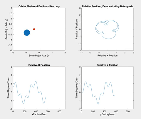
Below is the retrograde motion for Mercury. Due to its close proximity to Earth and its short orbital period, Mercury is retrograde about three or four times per one Earth orbit. These retrogrades are shown in the top right plot in each of the following figures. Having plotted relative position versus time, I wanted to see what would happen if I plotted the relative positions against each other. The resulting loops correspond to the inner planet lapping the outer planet, demonstrating the retrograde motion. These loops also correspond to the plateaus in the position versus time graphs.
Figure 7
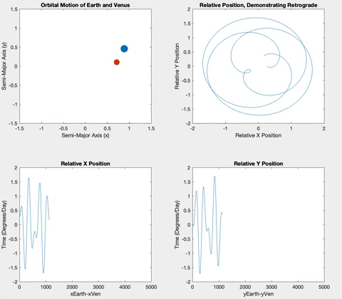
Venus and Earth are very similar both in their semi-major axis and in their period, resulting in fewer retrograde events in an Earth year.
Figure 8
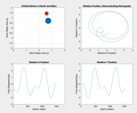
Mars is the first planet I simulated that is further from the Sun than the Earth itself, meaning the retrograde events occur when the Earth overtakes Mars.
Figure 9
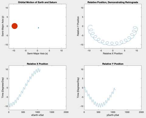
Further out in the solar system, both Jupiter (Figure 10) and Saturn (Figure 11) orbit very slowly compared to Earth. To capture the following gifs, I multiplied the relative degrees/day by 5. Without this factor, the motion of Jupiter and Saturn is almost imperceptible in the simulation. Their slow motion also make the retrograde motion much more regular and with a smaller precession because the outer planets move so much less as Earth travels around rapidly.
Figure 10

Figure 11
By allowing my simulation to run for larger multiples of pi, I could see the retrogrades precess with time and eventually meet up in the same place it began (because of the circular orbits).
Figure 12. Mercury retrograde after 100π

Figure 13. Venus retrograde after 100π

Figure 14. Mars retrograde after 100π

Figure 15. Jupiter retrograde after 200π

Figure 16. Saturn retrograde after 500π

Putting together the code for the orbits of Mercury through Mars resulted in the following, which I allowed to run for 100π (Figure 18). The result greatly resembles historical illustrations of epicyclical orbits, such as the image found here.
Figure 17
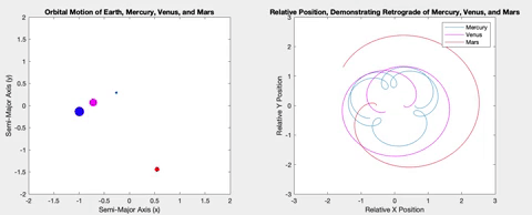
Figure 18

And finally, adding the last two planets and running the program (overnight) for 200π resulted in the following:
Figure 19

