
Background
In PHYS 375 we have studied several applications for numerical methods in solving otherwise impossible, or at least prohibitively difficult, differential equations. One example involved the Euler-Cromer method for solving the equation of motion for a pendulum both damped by atmospheric elements and driven by an outside force. At the most basic level, the equation of motion for a rocket can be treated in the same way as the damped driven pendulum — both are affected by three forces: gravitational force, a damping drag force, and a driving force. In the case of rocket motion, these forces are represented by the rocket’s weight, atmospheric and wave drags, and its thrust force. The biggest difference between the two problems is that because a rocket’s thrust force is much larger than any damping forces, it will not exhibit chaotic motion like the pendulum.
The equation of motion for a rocket is therefore:
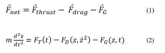
In this article I will explore each term of the equation of motion, covering the various dependencies that must be accounted for in the code, as well as any assumptions or simplifications made. Finally, we will see the results of this simulation for different rocket models.
I. Thrust Force
The majority of all rockets which have entered into orbit have been liquid-fuel rockets, as opposed to solid-fuel rockets (the notable exception being the Space Shuttle, which uses both). For a liquid-fuel rocket, thrust would be controlled during the ascent by a throttle, responding to rocket performance and adjusting thrust over time to control the trajectory. For the sake of the project, we are assuming that the thrust of the model rocket is constant for the duration of the ascent. A mathematical representation of the thrust force could be:
![]()
In other words, the thrust force is a constant up until the time at which the rocket runs out of fuel, after which it is zero. The constant value of the thrust will be known for each rocket model used in the simulation. Therefore: the thrust force is dependent on time only.
It is important to note that this model is purely one-dimensional. In a realistic rocket flight, the rocket would launch perpendicular to the surface, and then rotate by a small degree in flight to begin forming a parabolic trajectory. Therefore the actual vertical component of the thrust would be slightly lower than it is here. However, we can also assume that a rocket flying at any non-zero angle would generate a small amount of aerodynamic lift that would counteract this reduction in vertical thrust.
II.1 Atmospheric Drag
The drag acting on the rocket can be separated into two components: atmospheric drag and wave drag. Atmospheric drag, a form of parasitic drag, is a damping force opposite to the rocket’s motion due to skin friction between the surrounding air molecules and the surface of the rocket. The equation for drag force due to atmospheric skin friction is:
![]()
where ρ is the air density (kg/m3), v is the velocity of the rocket, CD is the drag coefficient, a A is the cross-sectional area of the rocket. The diameter of each rocket is given, so A will be known. The drag coefficient is difficult to determine without making physical tests on the rocket, but we will assume a value of CD = 0.75, which represents a flying shape somewhere between a cylinder and a cone. This is a relatively high drag coefficient; airfoils, for comparison, have values of CD well below 0.05.
Air density is more complicated to calculate, because it will decrease exponentially as the rocket ascends through the atmosphere. For altitudes under 86 km (the troposphere, stratosphere, and mesosphere), the air density can be given by the ideal gas law (Eq. 5). Here, R is the gas constant (8.314 J⋅K−1⋅mol−1) and M is the molar mass of air (0.029 kg/mol). Atmospheric temperature and pressure are also dependent on altitude, and are given by the barometric equations below.
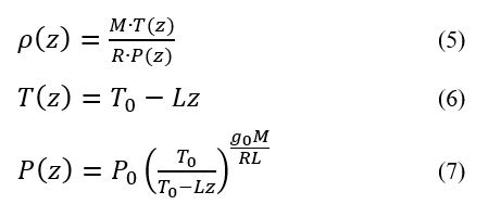
Here T0 and P0 are the baseline temperature and pressure for certain altitude regions, L is the temperature lapse rate for that region, and g0 is the acceleration due to gravity at sea level (9.81 m/s2).
Above 86 km, in the thermosphere, temperature rises more quickly because the atmosphere no longer shields the space from the sun’s rays. Pressure and air density, now very small, drop off with a quartic relationship to altitude.
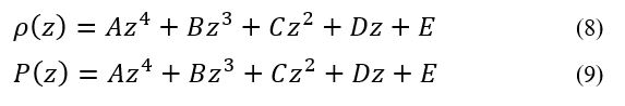
The coefficients of each term vary in different high-altitude regions. For a table of these coefficients, as well as the values for T0, P0 and L, please refer to this comprehensive mathematical model of the Earth’s atmosphere.
To correctly calculate atmospheric drag in my rocket simulation, I needed to write a function that could accept a value for altitude and compute the pressure, temperature, and air density in each atmospheric region. Here is this function, which stops distinguishing very small values for air density above z = 150 km. Running this function for increasing altitude produced the following graphs of temperature, pressure, and air density.

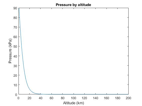

In summary, the code must update values of air density and drag within the for-loop of the Euler-Cromer method, because the atmospheric drag depends on both altitude and velocity.
II.2 Wave Drag
Earlier versions of my project failed to account for wave drag, or the drag force exerted on an aircraft by the pressure due to compressed waves of air. This force comes into play once the rocket exceeds its critical Mach number (typically Mach 0.8), and approaches the sound barrier. When an object approaches the speed of sound, it begins to move faster than the air waves in front of it, causing a rapid rise in drag. The peak in drag at Mach 1 causes the sound barrier, which is the primary obstacle for rockets attempting to leave the Earth’s atmosphere. When I did not account for wave drag in my simulation, rockets were able to reach space up to distances of 1,000,000 meters without difficulty.
Exact calculations of the relationship between drag and Mach number are difficult and rely heavily on the specific shape of the rocket. Furthermore, most information available on calculating wave drag is from the field of aerodynamic engineering, which deals in airplanes, not rockets. One equation, however, the Prandtl-Glauert Rule, can help approximate the effects of transonic drag forces in my rocket simulation.
The use of the Prandtl-Glauert Rule in this context requires several further caveats. First, it is currently accepted that the Prandtl-Glauert Rule is not valid for accurate calculations in the transonic region, only being valid for Mach numbers below 0.8 and between 1.2-5. I am choosing to ignore this disclaimer, because the rule in this region approximates the effect of the sound barrier well enough for the purposes of the project. Also, the Prandtl-Glauert Rule has been shown in experiments to underestimate increases in wave pressure (NACA Report No. 646, 1939). Two updates exist to the rule — the Karman-Tsien Rule, and Laitone’s Rule — which include higher-order terms. Lastly, the explicit definition of the Prandtl-Glauert Rule relates Mach number to the pressure coefficient of an aircraft, not its drag coefficient. Its application here is by analogy, noting the similar effects in equations for the Prandtl-Glauert corrections to coefficients of lift and moment.
The Prandtl-Glauert Rule (Equation 10) states that when dealing with compressible fluids, the aerodynamic coefficients (e.g. pressure, lift, drag, etc) must be divided by β, the Prandtl-Glauert Factor, which depends on the freestream Mach number. The Mach number is defined as the ratio of velocity over sound speed, and the sound speed in turn depends on air temperature.

In aerodynamics, in is customary to perform calculations using a frame of reference that moves along with the aircraft. The subscript ∞ below the Mach number, velocity, and sound speed (a) refers to the “freestream” value of each, meaning the speed of the moving air around the stationary vessel in this frame of reference, but far away from the vessel, where the shape of the aircraft can not yet affect the airflow. In Equation 13, γ is the ratio of specific heats (about 1.4 on average), and Rsp is the specific gas constant (287 J⋅kg−1⋅K−1 for dry air). For Mach numbers higher than 1 (supersonic speeds), the terms under the square root in Equation 11 are reversed.
We have previously established that air temperature depends on altitude, so we can say that wave drag depends both on velocity and altitude just as atmospheric drag does. For this reason, I also needed a function that could update the coefficient of drag at each iteration of the main for-loop.
Running the function at a fixed altitude and temperature for increasing rocket velocities produced the following results for wave drag:
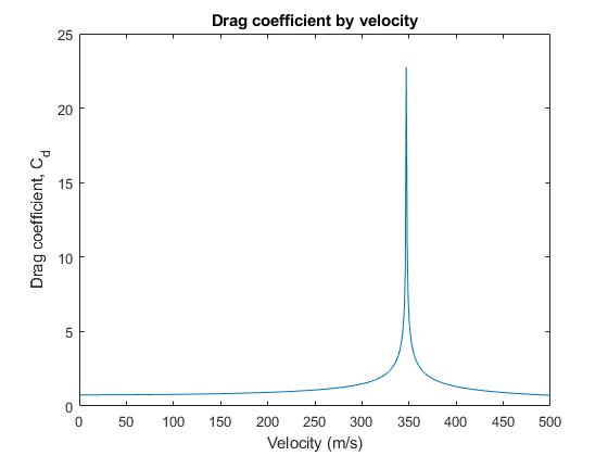
The drag peaks at 347.18 m/s, the speed of sound at 300 K. Notice that if that code had not corrected it, the drag would have been infinite at Mach 1 following Equations 10 and 11. This is called the Prandtl-Glauert Singularity.
III. Gravitational Force
The force due to gravity is given by the same simple equation as in other projectile physics problems: FG = mg. However, in this case, calculating the gravitational acceleration and the mass of the rocket introduces new problems.
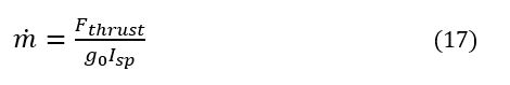
The mass of the rocket will always be decreasing as it expels fuel. Continuing to assume constant thrust, and therefore a constant mass flow rate out of the rocket, we can model the mass of the rocket with a linear time dependence as in Equation 15. The gravitational acceleration at an altitude z from the Earth’s surface is given in Equation 16, where RE is the radius of the Earth (6,371,000 m) and ME is the mass of the Earth (5.972 x 1024 kg).
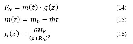
The mass flow rate can be calculated from the Tsiolkovsky Rocket Equation, given the thrust force and the specific impulse of the rocket. The specific impulse, in seconds, is a measure of the efficiency of the rocket’s engines, and is known for most rockets.
Because mass is decreasing over time, and gravity is decreasing with altitude, gravitational force depends on time and altitude.
We have now reduced the equation of motion to depend only on time, altitude as a function of time, and velocity (the derivative of altitude) as a function of time. We can now apply the Euler-Cromer method to solve for altitude and velocity and determine the rocket’s one-dimensional trajectory.
IV. Computational Method
My code for solving the equation of motion is attached here in full. A pseudo-code summary of the program is given below.
• Initialize universal constants (G, M_earth, mol, R, P0, T0, rho0, g0)
• Initialize rocket specifications (thrust, drag coef., diameter, area, wet and dry mass,
  specific impulse, mass flow rate)
• Euler-Cromer method
   ‣ initialize altitude (1 m), velocity (0 m/s), mass (m0), air density (rho0), and
     gravity (g0)
   for t from 0 to tmax
   ‣ update gravity, g(z)
   ‣ update mass, m(t)
   ‣ call density function, [rho,T,P] = f(z)
   ‣ call wave drag function, Cd = f(v,T,C0)
   ‣ calculate thrust force, FT(m)
   ‣ calculate drag force, FD(rho,v,Cd,m)
     if [drag vector condition]
   ‣ Euler-Cromer:  v = v + (thrust - drag - g)*dt
                    z = z + v*dt
   ‣ save matrix values for v, z, m, g, thrust, drag, and rho
   ‣ save end time
     if [crash condition]
     if [empty condition]
   end

• Plot z vs. t, v vs. t
• Plot FT, FD, and g vs. t
• Define density function, [rho,T,P] = f(z)
• Define wave drag function, Cd = f(v,T,C0)
I would like to call attention to the three “if conditions” in the for-loop, which were inserted as the result of trial and error. First, the “drag vector condition” is necessary because the code cannot determine the direction component of the velocity vector, only its magnitude. If the rocket fails, and begins to fall, the other forces will still point upwards, but the drag force will need another line of code to tell it to change sign when the velocity is negative.
The “crash condition” simply says to stop the for-loop and end the simulation when the rocket hits the ground, when z = 0 or z < 0. Otherwise, the rocket would fall through the Earth. This is also why the rocket’s altitude was initialized at z = 1, so as not to prematurely trigger this condition.
Finally, the “empty condition” says to set the thrust and mass flow rate equal to zero when the rocket runs out of fuel. The empty mass (“dry mass”) of the rocket was initialized, so the condition simply checks to see when m = mdry. When I had not yet written this condition, the rocket’s mass would decrease to negative infinity.
V. Results, Single-Stage Rocket
The test rocket used in the simulations was the Falcon 1e, a theoretical rocket designed by SpaceX in 2011 as an update to the earlier Falcon 1. The Faclon 1e was never launched, which gave me the inspiration to test its theoretical viability in my simulation. The Falcon 1e specifications, compared to other rockets which I tried in the simulation, are given below.
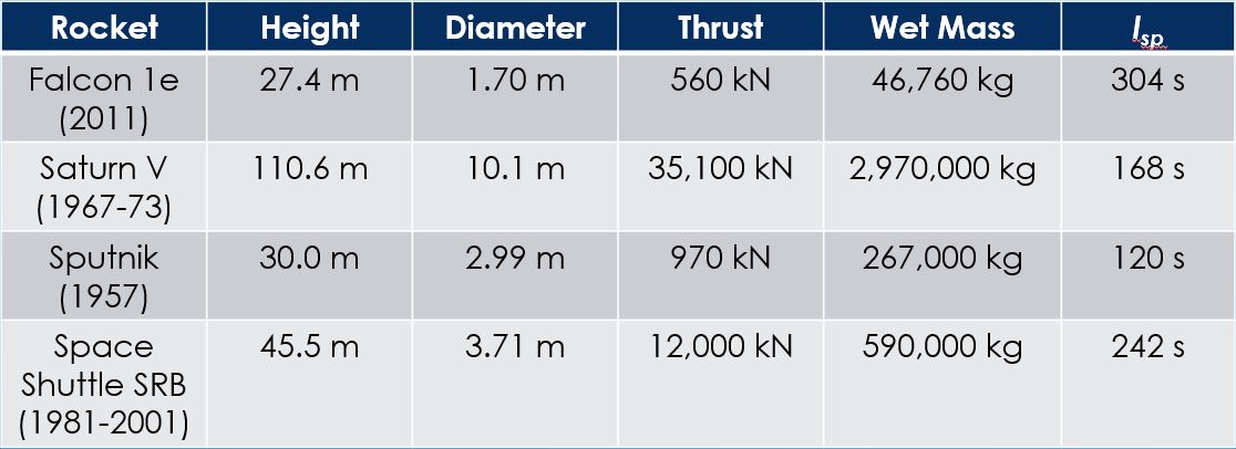
The next two figures show the rising altitude and velocity of the rocket, as well as the relative strength of each component force over time.


We can see that the Falcon 1e will fly for about 169 seconds before it runs out of fuel and the thrust force drops to zero. By that time it has reached an altitude of about 125 km, still short of the 200 km required for a comfortable low-earth orbit. This is consistent with our expectations: no single-stage rocket in history has every made it to orbit from Earth. The topic of a single-stage-to-orbit spacecraft (SSTO) is an area of current research, mostly among defense contractors.
The flatline in the velocity curve around 65-95 seconds represents the rocket approaching the sound barrier. The corresponding sudden increase in drag represents effects of compressibility and wave drag taking hold. Note how the graph of drag directly across the sound barrier around 95 seconds seems to exhibit more erratic, possibly chaotic fluctuation. This occurs because thrust and drag at this point in time are competing for dominance over the rocket’s net force. Once the sound barrier is breached, drag quickly becomes negligible, as the air waves move behind the rocket, and air density becomes very thin. Making the jump to supersonic speeds, therefore, is critical in order to leave the Earth’s atmosphere; although the jump requires a high amount of thrust and a sturdy spacecraft, choosing to remain at subsonic velocities would be less effective overall due to the higher drag on the rocket.
VI. Results, Two-Stage Rocket
In order to get to space, our simulated rocket will need two stages. Specifications for both stages of the Falcon 1e are public on Wikipedia and the SpaceX website. In order to achieve this in the code, I added the following lines inside the for-loop:
 if z < 0              % rocket crashes or fails to launch
        break
    elseif m < empty      % rocket runs out of fuel, mass becomes stable
        FT = 0;
        dm = 0;
        nextstage = nextstage + 1;
    end

    if nextstage == 15
        nextstage = 0;
        break
    end
In other words, when the rocket runs out of fuel, the program will continue for another 15 iterations of the loop, and then will break (nextstage was initialized as zero). After that, I reinitialized the specifications of the rocket for its second stage and then ran a second for-loop identical to the first, but without reinitializing the holding matrices for the variables.
The results for the two-stage Falcon 1e’s altitude trajectory, velocity, and force diagrams are shown below. The program was instructed to stop when the rocket reached an altitude of 250 km.


We can see that the first stage did most of the hard work. After crossing the sound barrier, very little additional thrust or increase in velocity was needed to complete the journey to space. This is because, as previously mentioned, the drag at high altitudes and supersonic speed is negligible. We can also see that the second stage of the rocket did not expend all of its fuel. This is necessary, because once the rocket has escaped the Earth’s atmosphere, the second (or third) stage will still be responsible for making orbital maneuvers in space. For example, if the rocket’s mission is to launch a satellite, or rendez-vous with the International Space Station, the rocket will need to rotate parallel to the surface of the Earth and increase its velocity to around 7.8 km/s, the normal minimum velocity for low-earth orbit. For comparison, this speed at sea level would correspond to nearly Mach 23. My simulation of the Falcon 1e only achieved 3.8 km/s, or Mach 11 at sea level, during its ascent.
References
[1] Anderson, John D. Fundamentals of Aerodynamics. 5th ed. New York: McGraw-Hill, 2011.
[2] Braeunig, Robert A. Basic of Space Flight: Atmospheric Models. 2014. http://www.braeunig.us/space/atmmodel.htm.
[3] Giordano, Nicholas J., and Hisao Nakanishi. Computational Physics. 2nd ed. Upper Saddle River, NJ: Pearson Prentice Hall, 2006.
