What is Positron Emission:

Positron emission is a type of radioactive decay also referred to as beta positive decay. It occurs when a proton in a nucleus is converted into a neutron and a positron is emitted, as well as an electron neutrino. A positron has the mass of an electron with a positive charge. Figure 1 shows this process.

Figure 1. Example of positron emission. Made using Microsoft Word.

This project will simplify the process of positron emission by solely focusing on the proton to neutron conversion using a quantum potential well. Now how does the potential well represent this nuclear reaction? Figure 2 shows the model of the simplified potential well that this project will use in the MATLAB simulations.

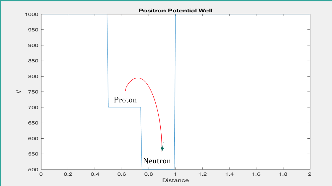
Figure 2. Positron Potential Well. Created using MATLAB.

First, we must understand that at short distances between particles the nuclear strong force binds the particles and their motion. At long distances between particles, the Coulomb interaction predominates. The nuclear force is very attractive and much stronger than the Coulomb force. Thus, these two forces have very different levels of potential energy. If a nuclear decay has enough kinetic energy to overcome the Coulomb repulsion it releases energy and the particles drop into a deep attractive well. The greater the kinetic energy of the decay and the lower the barrier the more likely the particles are to tunnel through the barrier. The size of the barrier depends on the specific reaction. The final energy state is different for each positron emission depending on the nucleus that is decaying. This process can occur in many different elements and isotopes.  Thus, this project does not use a specific energy level but generalizes to reasonable values. The probability of a particle to decay has a strong dependence on the number of protons in the initial particle. In addition to the strong nuclear force and the coulomb force, the electromagnetic force is important for understanding positron emission. The electromagnetic force only acts on the protons, not the neutrons, in the nucleus of a particle because these are the particles that contain a charge. This is the reason that a nuclear potential well, such as positron emission, will look different than other potential wells we may have seen in early physics textbooks. This project will further simplify this model to have an equal number of protons and neutrons in the decaying particle initially. This is of course not always the case in these reactions. The difference in well depth for protons and neutrons in a potential well is why light nuclei usually have equal numbers of protons and neutron while heavier nuclei have more neutrons.

A bit about Quantum Tunneling:

This project already has a vast scope of physics it is covering but I thought it was important to touch upon quantum tunneling. Quantum tunneling occurs when a particle penetrates a barrier of potential energy with a height greater than the energy of the particle’s wave function. This project will use finite quantum wells rather than infinite so the particle has the ability to penetrate the barrier. The particle’s ability to penetrate the barrier depends on the incident energy of the particle. The energy of the particles before and after tunneling can be expanded upon using the Time-Independent Schrodinger Equation (TISE) which will be discussed later in this project. The ground state solution to the TISE is the lowest even parity state that can be expressed by the TISE. Even parity wave functions are symmetric. The positron emission has different sizes of potential wells based on the number of neutrons and protons and is thus not symmetric. We must look at energy values that are higher or lower than the ground state for our wave function. This is where Figure 3 comes in. If the energy of the particle is higher than the ground state energy of the symmetric well, the wave function will drop at the barrier; tunneling. If the energy of the particle is less than the ground state, the wave function will go to infinity at the boundary of the barrier; not tunneling.  If the energy was at the ground state, the wave function would go to zero. This project will exemplify different types of energy, greater than and less than the ground state, as well as equal to the ground state. Again, we will only use relative energy values because exact values depend on the type of emission. Using arbitrary energy values is still an effective model because it is more important to visualize energy larger or greater than the ground state. It does not matter so much what that ground state actually is unless you are doing a more complex project. Using specific energy values corresponding to actual decay reactions would be the next step in this project.

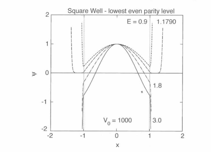
Figure 3. Energy levels relative to ground state for Finite Square Well. Computational Physics (2nd Edition) by Giordano, Nicholas J. and Nakanishi, Hisao.

Methods:

All of the following computational methods use the Time-Independent Schrodinger Equation. The finite difference method uses the TISE directly along with its derivative, while the matching and shooting algorithms use a discretized version of this equation. The derivation of the TISE into a discretized form is shown in the following Figure 4. All constants are simplified to the value 1. These methods will be further discussed in the following section.

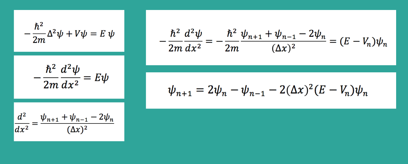
Figure 4. TISE derivation into discrete steps for solving for the wave function. Start at top left and move down and then continue at top right and down. Equations made in Microsoft Word and background from Google Slides.

The finite difference algorithm was used first to model a non-positron emission potential well. This well has only one potential energy drop. The steps to this method are as follows. Set boundary conditions. Choose central, forward or backwards finite difference method depending on availability of boundary conditions. Forward finite difference uses the boundary condition at the beginning of the problem; the initial state of the wave function. Backward finite difference uses the boundary condition at the end of the problem; the final state of the wave function. Central finite difference uses the center wave function value to the find the other corresponding energy values. Take the derivative at each point in the space iteration. Iterate over matrices instead of points for 2D or 3D. This project is just in 1D, but it is interesting to note other possible applications to this method. Use the derivatives to form a Taylor series and approximate the original solution from that. The result of this method is shown in Figure 5 for a non-nuclear potential well. This well has even parity and is symmetric on both sides. The wave function is cut off at the sides and tunneling is ignored because this was a first step to understand modeling potential wells in general. Tunneling will be touched upon later. The MATLAB trapezoid function was used to find the derivatives.

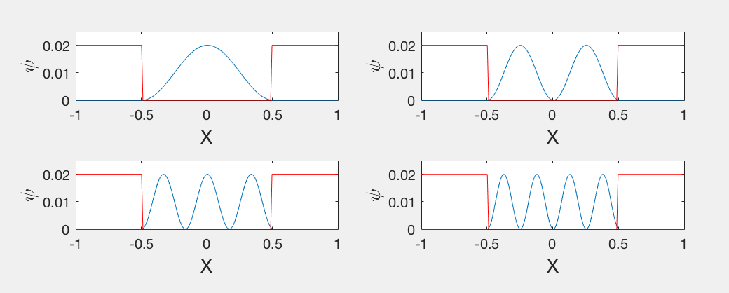
Figure 5. Finite Difference Method for non-positron emission. Produced using MATLAB.

Next, the shooting method was used. This method requires the first and last boundary conditions of the problem to be identical and thus is only to be used with even parity potential wells. This was modeled for non-positron emission but added the tunneling effects. So the wave function’s behavior after the potential barrier is included. In Figure 6 there is a drop in the energy of the wave function at the potential barrier so tunneling is taking place. The drop here is very dramatic and may not be realistic as the wave attenuates into the barrier, but it is acceptable for our purposes. We are able to see the behavior of the wave function change drastically at the barrier when the energy is less than the ground state energy. The ground state energy used here as an example was 1.23 MeV. The steps of the shooting method are as follows. Set boundary conditions on each side of the interval. Must have even parity. Make an initial guess at the value and plug it into the differential equation. Check the solution with the final boundary condition. If they don’t match, try the next value using the given time step.

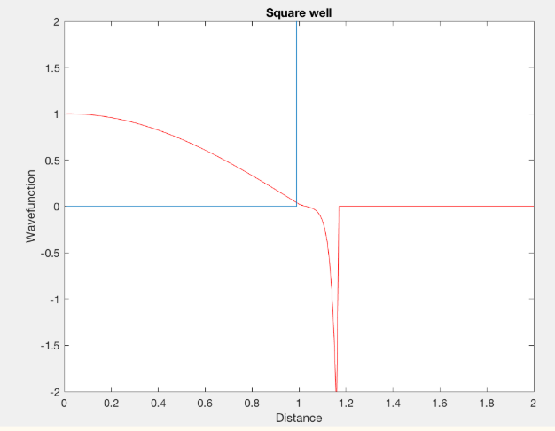
Figure 6. Non-positron Emission Potential Well. Particle initial energy greater than ground state energy. Created with MATLAB.

The third and final method used in this project was the matching method. The steps for this method are as follows. Boundary conditions set at the left and right sides. Iterate over the differential equation from the left and again separately from the right. Choose a matching point at which both sides have the same value and continuous slopes. Adjust the values for given time steps until the matching point is correct. This was the most accurate method to model positron emission. Figure 7 shows the particle tunneling in the barrier. This problem is interesting because there is a spike in the wave function energy at the exact point that the proton would decay into the neutron. This represents the emission of the positron. This spike in energy gives the particle the energy to overcome potential barrier and continue until its eventual attenuation in the finite well. Figure 6 shows two identical graphs, one calculated from the leftmost boundary condition and one calculated from a rightmost boundary condition. An algorithm for the matching point was used to only display the wave form only when the two calculations, one from each side, were identical.

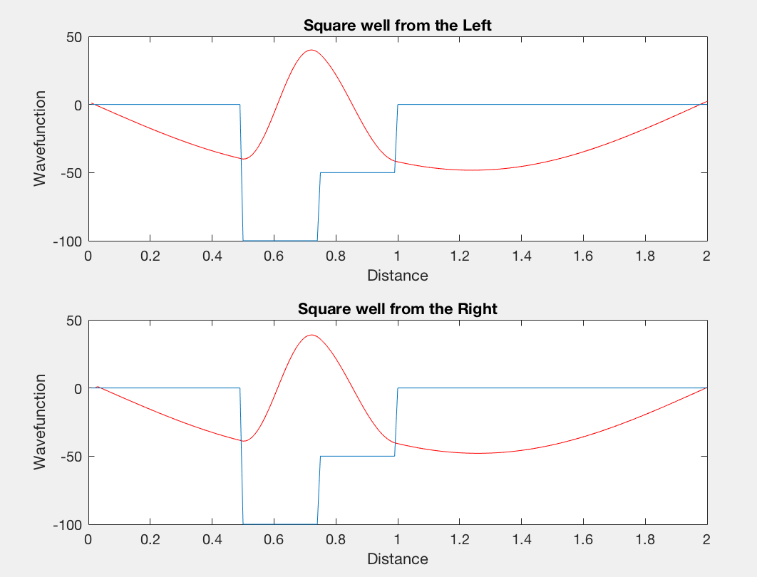
Figure 7. Positron Emission potential well using the matching method. Created using MATLAB

Future Work and Applications:

Positron emission is very important in industry because of its application to medical imagining. Positron Emission Tomography (PET) scans are a form of medical imaging in which photons are produced by the annihilation of a positron (through beta plus decay) and an electron through decay of certain isotopes. These photons can then be detected and imaged. The matching, finite difference, and shooting methods can also be applied to a myriad of quantum mechanics problems. These computational methods can be used with the harmonic oscillator, different nuclear reactions, spherical harmonics, Lennard-Jones potential and more. This project can be improved by modeling a specific particle and its potential energy levels as well as decay energy levels. This would give the program specific numbers for energy instead of using arbitrary values. Another way to improve this project would be to try a negative beta decay example and make sure the methods still work. It would also be helpful to have gif animations of the methods. This was a very interesting project because I have worked with nuclear physics in my summer internships but never in a MATLAB setting. I came into this class as a novice at MATLAB and I feel confident that my abilities have improved.