Background:
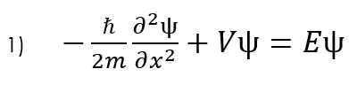
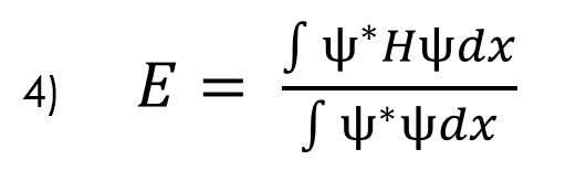
Photobleaching is the photochemical alteration of a dye or fluorophore molecules that removes its ability to fluoresce. This is a chemical reaction initiated by the absorption of energy in the form of light, with the consequence of the creation of transient excited states with differing chemical and physical properties1. It most commonly occurs in fluorescence microscopy, where the over excitation of the material or overexposure causes the fluorophore to permanently lose its ability to fluoresce due to the photon-induced chemical damage and covalent modification2. However, scientists have newly developed the ‘bleaching-assisted multichannel microscopy’ (BAMM) technique which allows them to manipulate the rate of photobleaching in order to help differentiate fluorophores3. Because the overcrowding of fluorophores attached to different cell targets prove to be a major limitation in imaging, this technique allows researchers to use photobleaching to differentiate between fluorophores rather than the current technique that relies on the different fluorescent emission colors for labelling. The varying rates of photobleaching, or photostability, for the different types of fluorophores allows for this new kind of differentiation. The once weakness of the fluorescent microscopy process is now seen as a strength that allows for increased identification of cellular targets.
Most students are introduced to photobleaching in introductory Biology courses, where the process is exploited to study the diffusion properties of cellular components in molecules by observing the recovery or loss of fluorescence to a photobleached site. The observed changes are due to the change of states from electron excitation via intersystem crossing. Studying the movement of electrons via transitions from the singlet state to the triplet state gives us a better conceptual grasp on the photobleaching process with a molecular focus on energy levels and the wavefunctions of the different spin states. The selection rules describe whether a quantum transition is considered to be forbidden or allowed. This means that not all transitions of electrons are observed between all pairs of energy levels, with “forbidden” being used to describe highly improbable transitions. I will further explore what it means for electrons to change state and which kind of transitions are more probable than others by studying the selection rules and the principles that support their claims. The applicational experiment that I performed, the photobleaching of methylene blue, demonstrates these reactions in real time through color intensity observations.
The Selection Rules
The Laporte Selection Rule
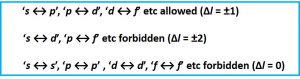
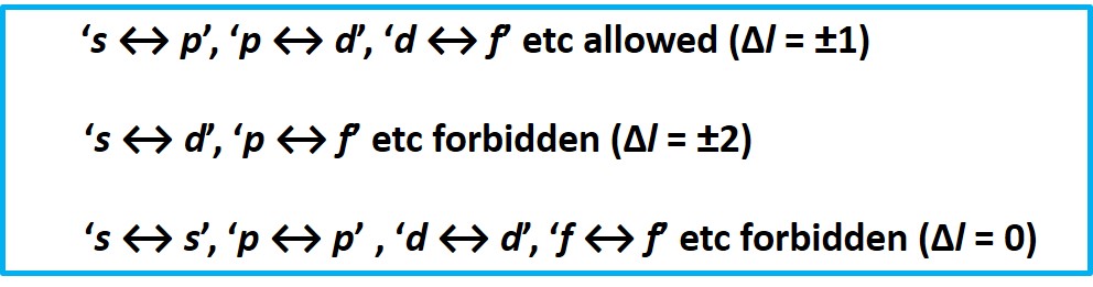
The Laporte selection rule states that the donor orbital and acceptor orbital of the electrons in a transition must have different symmetry or cannot be of the same orbital: (s →s); (p →p); (d →d); (f →f). Additionally, the Laporte allowed transitions allow for (Δ l = ± 1) changes in angular momentum quantum number (1).
 (1)
(1)
It indicates that transitions with a given set of p or d orbitals are forbidden if a molecule has a center of symmetry or is centrosymmetric. The selection rule determines whether the transition is orbitally allowed or forbidden. If the integral of the transition moment does not contain the totally symmetric representation, the transition is forbidden.
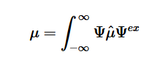
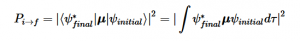
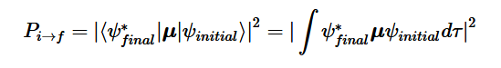
Transitions are only detectable when the transition moment dipole is nonzero and when the wavefunctions include the initial and final states which contain both the electronic and nuclear wave functions (2). The Born-Oppenheimer approximation points out that electronic transitions have a much smaller time scale than nuclear transitions; because of this and the fact that these transitions in question are electronic, the nuclear motion is ignored (3). This approximation is done because we assume that these transitions are instantaneous, so there is no change in the nuclear wavepacket. The Franck-Condon principle is a direct consequence of this approximation, which will be further explored later.
 (2)
(2)
 (3)
(3)
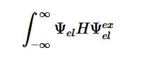
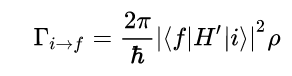
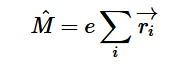
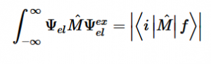
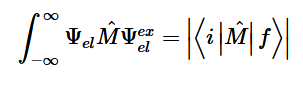
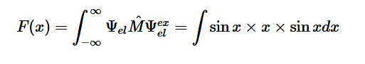
Fermi’s Golden Rule (4), which describes the transition rate or probability of transition per unit time from one eigenstate to another and is only allowed if the initial and final states have the same energy, allows M, the electric dipole moment operator to replace the time dependent Hamiltonian (5), giving that final transition moment integral that describes electronic transitions from ground to excited states (6). This integral is equivalent to the probability of a transition taking place. Since the integral must be non-zero for the transition to occur, the two states must overlap, as per the Franck-Cordon principle which states that the probability of electric transition is more likely if the wavefunctions overlap.
 (4)
(4)
 (5)
(5)
 (6)
(6)
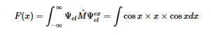
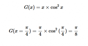
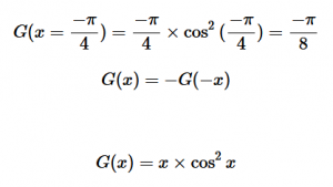
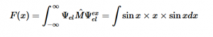
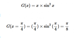
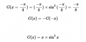
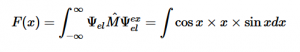
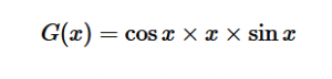
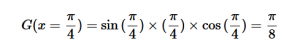
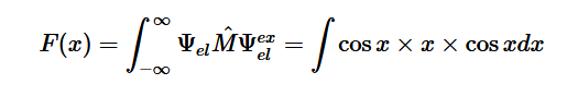
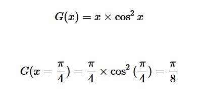
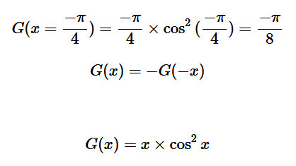
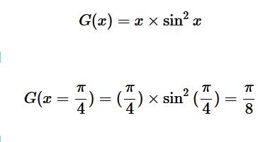
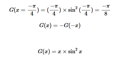
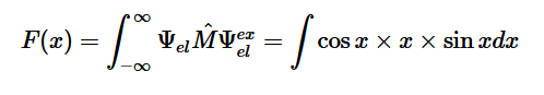
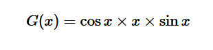
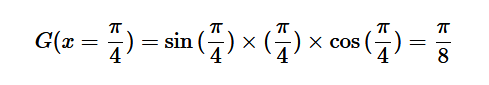
For solving the transition moment integral, the electric dipole moment operator can be rewritten with Cartesian axes (7). Simulating calculations of transitions with M being an odd function between even states (8) , between odd states (9), and even and odd states (10) show that transitions between two similar states are forbidden since the final result is an odd function. Even functions may be allowed transitions but to determine which are totally symmetric, cross products between the initial and final states with the electric dipole moment operator should be worked out.
 (7)
(7)
Two even states:
 (8)
(8)
Two odd states:
 (9)
(9)
One even and one odd state:
 (10)
(10)
Spin Selection Rule
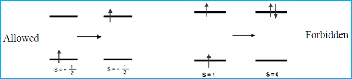
The spin selection rule states that the overall spin S of a complex must not change during an electronic transition (Δ S=0) or (Δ mS = 0). The spin state or spin of the excited electron coincides with the number of unpaired electrons; the singlet state having zero unpaired electrons and triplet state having two unpaired electrons. The overall spin state must be preserved, so if there were two unpaired electrons before transition, there must be two unpaired electrons in the excited state as well (Figure 1).

Figure 1: The allowed transition shows the transition of states in which the spin remains the same, with one unpaired electron on either side, a doublet to a doublet state. The forbidden transition shows the transition of a triplet state, where there are two unpaired electrons to an excited singlet state where there are no unpaired electrons. The loss of preservation of spin state of the molecule makes the transition forbidden.
The absorption of higher frequency wavelengths, which come in the form of photons or other electromagnetic radiation, excite electrons into higher energy levels. Electrons in general occupy their own states and follow the Pauli Exclusion Principle, which states that no two electrons in an atom can have identical quantum numbers and only two can occupy each orbital but must have opposite spins. The Exclusion Principle acts primarily as a selection rule for non-allowed quantum states. Equation 11 shows the probability amplitude that electron 1 is in state “a” and electron 2 is in state “3”, but fails to account for the fact that electrons are identical and indistinguishable. We know that particles of half-integers must have antisymmetric wavefunctions and particles of integer spin must have symmetric wavefunctions. The minus sign in equation 12 serves as a correction to equation 11. This new equation indicates that if both states are the same, the wavefunction will vanish, since both electrons cannot occupy the same state.
Ψ= Ψ1(a) Ψ2(b) (11)
Ψ= Ψ1(a) Ψ2(b) Ψ ± Ψ1(a) Ψ2(b) (12)
Singlet to Triplet Transition
When an electron in a molecule with a singlet state is excited to a higher energy level, either an excited singlet state or excited triplet state will form. A singlet state is a molecular electronic state where all the electron spins are paired. An excited singlet state spin is still paired with the ground state electron. The pair of electrons in the same energy level have opposite spins as per the Pauli exclusion principle. In the triplet state, the spins are parallel; the excited electron is not paired with the ground state anymore. Excitation to the triplet state is a “forbidden” spin transition and is less probable to form. Rapid relaxation of the electrons allow the electrons to fluoresce and release a photon of light, falling down to the singlet ground state level, which is known as fluorescence.
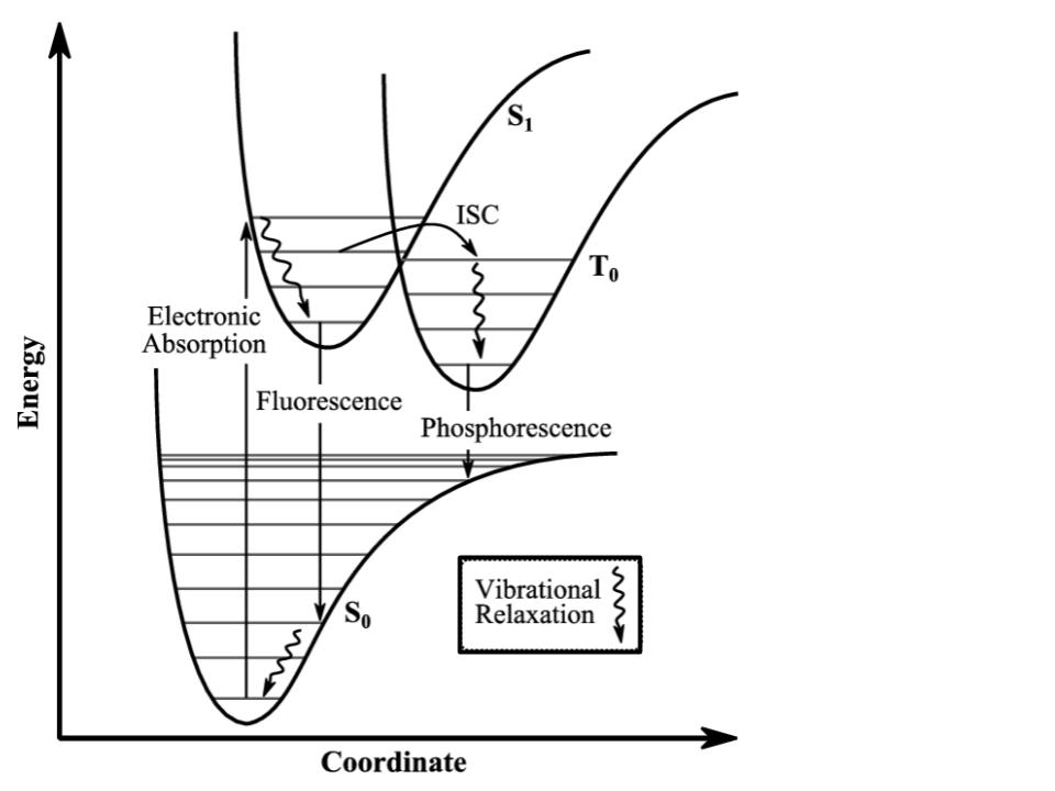
Intersystem crossing occurs when some molecules transition into the lowest triplet state which is at a higher spin state than the excited singlet state but has lower energy and experiences some sort of vibrational relaxation. In the excited triplet state, the molecules could either phosphorescence and relax into the ground singlet state, which is a slow process, or absorb a second phonon of energy and excite further into a higher energy triplet state. These are the forbidden energy state transitions. From there it will either relax back into the excited triplet state or react and permanently photo bleach. The relaxation or radiative decay of the excited triplet metastable state back down to the singlet state is phosphorescence where a transition in spin multiplicity occurs (Figure 2).
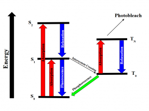
Figure 2: Energy diagram showing the transitions the electrons undergo when gaining and releasing energy. Although the first excited singlet state, S1, has a lower overall Spin State (S=0), the intersystem crossing shows that the triplet state has lower energy (S=1). The photobleaching pathway via the triplet state is highlighted as further excitations in triplet states are more likely to bleach fluorophores.
To further clarify, intersystem crossing (ISC) occurs when the spin multiplicity transforms from a singlet state to a triplet state or vice versa in reverse intersystem crossing (RISC) where the spin of an excited electron is reversed. The probability is more favorable when the vibrational levels of the two excited states overlap, since little or no energy needs to be gained or lost in the transition. This is explained by the Franck-Condon principle. States of close energy levels and similar exciton characteristics with same transition configurations are prone to facilitating exciton transformation4.
Zeeman Effect
Transitions are not observed between all pairs of energy levels. This can be seen in the Zeeman effect, a spectral effect, of which the number of split components is consistent with the selection rules that allow for a change of 1 for the angular momentum quantum number (Δ l = ± 1) and a change of zero or of one unit for the magnetic quantum number (Δ ml = 0, ± 1). The orbital motion and spin of atomic electrons induce a magnetic dipole, where the total energy of the atom is dependent on the orientation of this dipole in a magnetic field and the potential energy and orientation is quantized. The spectral lines that correspond to transitions between states of different total energy associated with these atoms are split because of the presence of a magnetic field5. This was looked for by Faraday, predicted by Lorentz, and observed by Zeeman.
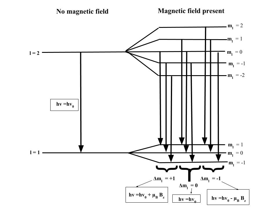
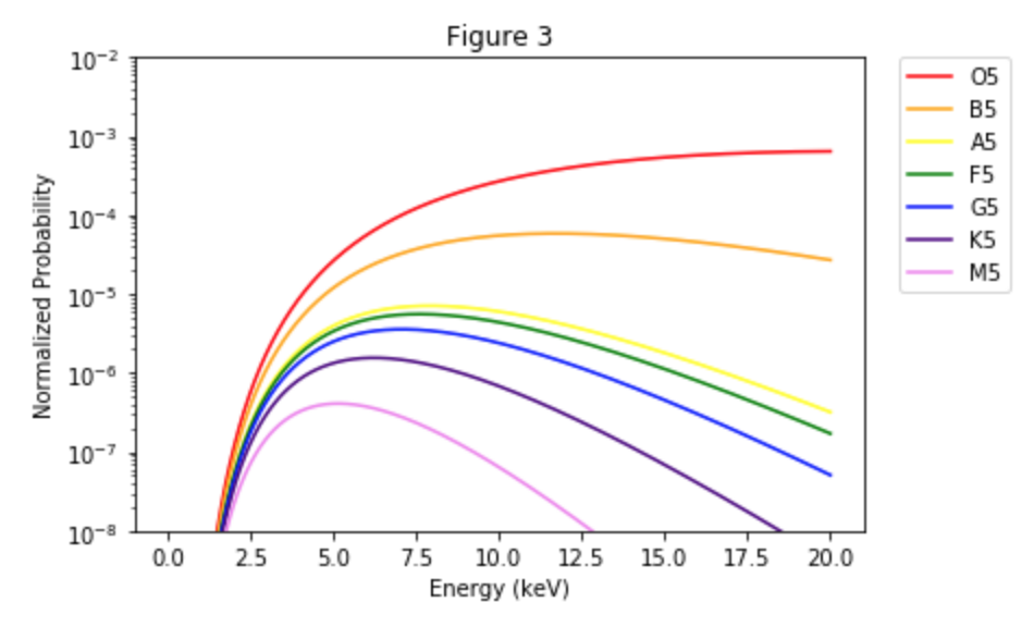
The Zeeman effect or “normal” Zeeman effect results from transitions between singlet states while the “anomalous” Zeeman effect occurs when the total spin of either the initial or final states is nonzero with the only tangible difference between the two being the large value of the electron’s magnetic moment of the anomalous effect. (Figure 3). For singlet states in the normal Zeeman effect, the spin is zero and the total angular momentum J is equal to the orbital angular momentum L. The anomalous Zeeman Effect is complicated by the fact that the magnetic moment due to spin is 1 rather than 1/2, causing the total magnetic moment (14) to not be parallel to the total angular momentum (13).

Figure 3: The normal Zeeman Effect occurs when there is an even number of electrons, producing a S = 0 singlet state. While the magnetic field B splits the degeneracy of the ml states evenly, only values of 0 and ± have transitions. Because of the uniform splitting of the levels, there are only three different transition energies.
 (13)
(13)
 (14)
(14)
Franck-Condon Principle
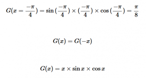
The Franck-Condon principle is a rule used to explain the relative intensities of vibronic transitions, in which there are simultaneous changes in vibrational and electronic energy states of a molecule due to the absorption of emission of photons. This principle relies on the idea that the electronic transition probability is greater if the two wave functions have a greater overlapping area. The principle serves to relate the probability of a vibrational transition, which is weighed by the Franck-Condon overlap integral (15), to the overlap of the vibrational wavefunctions.
 (15)
(15)


Figure 4: Energy state transitions represented in the Franck-Condon principle energy diagram. The coordinate shift between the ground and excited states indicate a new equilibrium position for the interaction potential. The shorter arrow indicating fluorescence into the ground state indicates that a longer wavelength and less energy than what was absorbed into the excited state.
Classically, the Condon approximation where there is an assumption that the electronic transition occurs on a short time scale compared to nuclear motion allows the transition probability to be calculated at a fixed nuclear position. Since the nuclei are “fixed”, the transitions are considered vertical transitions on the electronic potential energy curves. The resulting state is called a Franck-Condon state.
The nuclear overlap between state transitions can be calculated by using the Gaussian form of the harmonic oscillator wavefunctions.
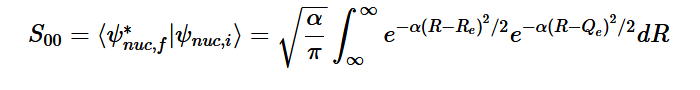
Overlap of Zero-zero transition S00
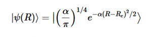
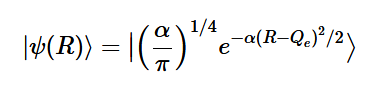
Using the harmonic oscillator normalized wavefunctions for the ground (16) and excited electronic states (17) where α = 2πmω/h, Re is the equilibrium bond length in the ground state and Qe is the equivalent for the excited state, the nuclear overlap integral can be determined (18). Expanding the integral and completing the square gives us equation (19). Simplifying the Gaussian integral gives us the overlap of the zero-zero transition states (20).
 (16)
(16)
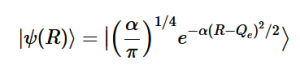 (17)
(17)
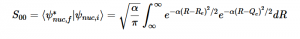 (18)
(18)
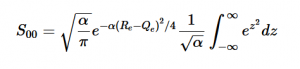 (19)
(19)
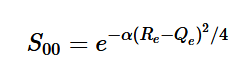 (20)
(20)
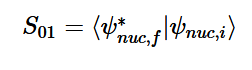
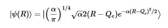
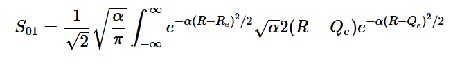
Overlap of S01 Transition
Solving for the zeroth level of vibration in the ground and the first excited vibrational level of the excited state, S01 is similar to how S00 was solved, using the equation (21) again. Using (16) and (22) as the zeroth and first excited state wavefunctions for the ground and excited states, the overlap can be found (23). Simplifying similarly to the previous walk-through, equation 24 shows the simplified overlap of the vibrational levels value.
 (21)
(21)
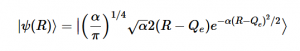 (22)
(22)
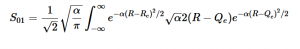 (23)
(23)
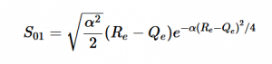 (24)
(24)
Applicational Experiment: Photobleaching of Methylene Blue
Experimental Background:
A HeNe laser emits a wavelength along the visible spectrum that is absorbed by the methylene blue causing a reaction known as photobleaching. The methylene solution will take on a colorless appearance due to the absorption of the photons, exciting the electrons into new spin state. A singlet spin state, which quantifies the spin angular momentum in the electron orbitals, will either transition into a ground state or into an excited triplet state, both of which have lower energies. The transition into the triplet state involves a change in electronic state which increase the states lifetime, allowing it to be a strong electron acceptor.
The colorless appearance of the irradiated solution is due to the oxidation of the triethylamine due to the excited triplet state. The ‘photobleaching’ of the methylene blue, as more easily seen from placing and removing the solution from sunlight, is not permanent and functions more as a decay in which the electrons jump to high energy excited states and fall back down to its ground state. Using a laser has a longer lasting effect on the solution, as more waves of higher frequency are absorbed, slowing down the time it takes for the solution to return to its original state.
Experimental Procedure and Results:
With supplies provided by the Chemistry department and Professor Tanski, I was able to create the methylene, triethylamine mixture. Triethylamine is a chemical that has a strong odor so working under a hood is essential. (Or else the whole building would have to evacuate cause of the smell if it fell!) While wearing googles in a chemical hood, I measured out 10mL of water with a graduated cylinder into a 10mL vial, added 1-2mg of methylene blue powder, which is such a small amount that it was very difficult to weigh out, and added 5 drops of triethylamine. I pipetted approximately 0.75mL of the sample into three 1mL vials, labelled for photobleaching by the red HeNe laser, green HeNe, or as the experimental control. The remaining liquid was meant to examine the effects of natural sunlight on the methylene solution. The dark blue solution was meant to lighten in color due to the suns less intensive photobleaching properties. Placing the solution back in darkness would allow for the excited electrons to fall back down to the ground state and return to its original color, since the energy absorbed wasn’t high enough to cause permanent photobleaching. For some reason, my solution did not have a reaction to the sun as expected, which was probably due to me not mixing the solution well enough before I distributed it into three other vials. In comparison to my predictions with the reactions using the HeNe lasers, the sunlight would take longer to turn colorless but would take a very short amount of time to return to its original color, since the excited electrons are not falling from a high energy level.
I then visited the Michelson Interferometer and Fourier Transform experimental set up that had the red and green HeNe lasers that I required. I darkened the room to lessen the effects of stray light, but since the shades don’t completely block out the sunlight, I couldn’t reach full darkness. With one laser on at a time, I placed the vial directly in front of the beam, hoping to irradiate the appropriate vial with the laser until the color changed. Unfortunate, my vials did not change color at all, even after holding them to the beam for thirty minutes straight. As I mentioned earlier, this error was probably due to my lack of proper mixing of the solution. What was meant to happen was that the energy received from each laser was supposed to turn the solution clear in color. I would have predicted that the red laser, due to higher frequency and higher energy in the photons, would have caused the solution to become colorless quicker and after keeping the vials in darkness, would take longer to return to its original dark blue color since the excited electrons have higher energy levels to fall from.
Overview:
Reproducing the photobleaching of methylene blue allowed me to apply my knowledge about the electron spin states, specifically singlet and triplet states, and the observable transitions that was suppose to take place in my experiment. I had learned a bit about spin states in Organic Chemistry but studying them from a Physics standpoint is very different, requiring further conceptual questioning about why certain transitions were more likely than others. My in-depth look into the rules and principles behind the seemingly simple excitation of electrons into different states was very interesting and a great experience, prying apart every argument, looking for the basis of which each statement came from, and learning the conceptual theory as well as the mathematics that back it up. Thank you Professor Magnes for a great semester!
(1) https://www.britannica.com/science/photochemical-reaction
(2) https://www.microscopyu.com/references/fluorophore-photobleaching
(3) https://phys.org/news/2018-06-fluorescence-microscopy-bamm-treatment.html
(4) https://www.ncbi.nlm.nih.gov/pmc/articles/PMC5524908/
(5)http://bcs.whfreeman.com/webpub/Ektron/Tipler%20Modern%20Physics%206e/More%20Sections/More_Chapter_7_2-The_Zeeman_Effect.pdf


 (6)
(6)
 (8)
(8)
 (9)
(9)
 (10)
(10)

 (15)
(15)


 (23)
(23)
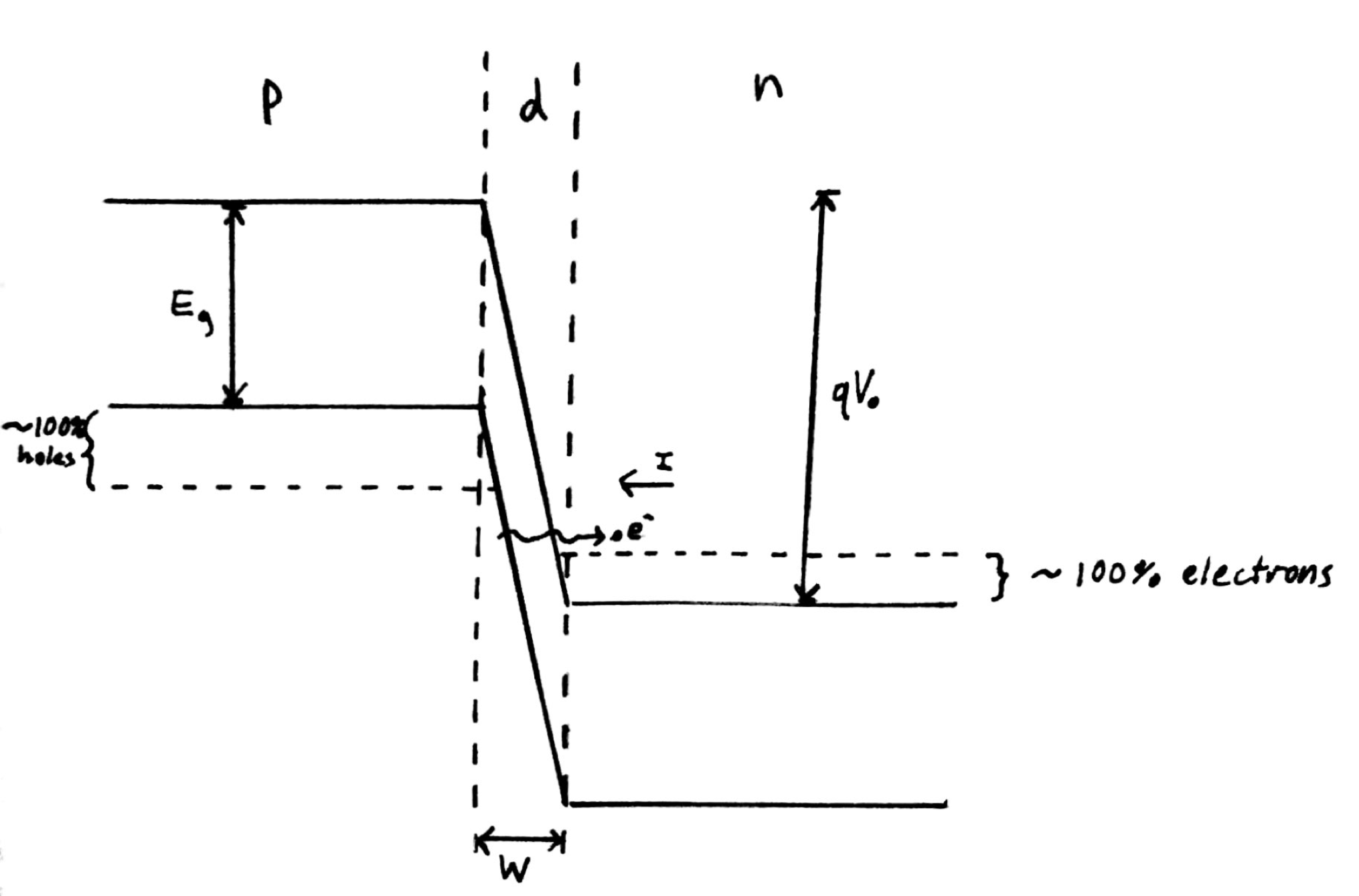 Fig. 1: Band diagram representing Esaki diode under tunneling condition. The diode is reverse biased, allowing an electron on the p side to tunnel across to an empty state on the n side.
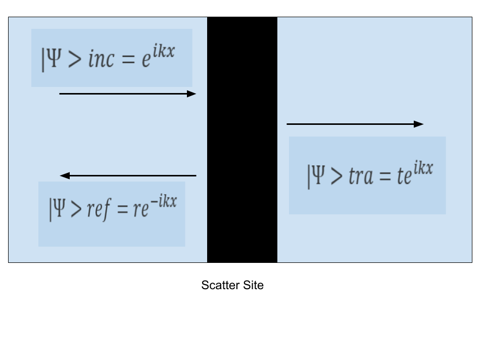
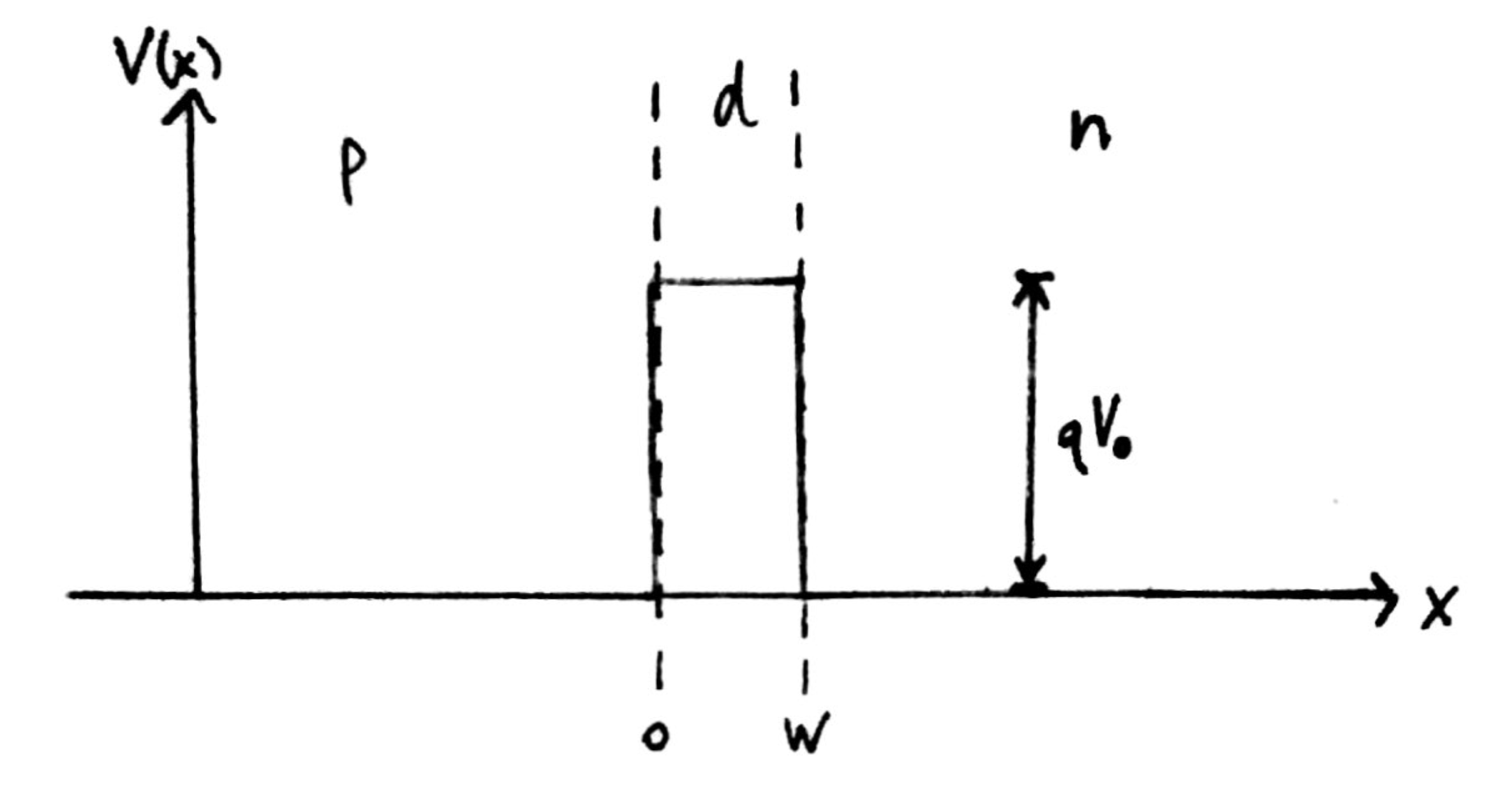 Fig. 2: Rectangular potential barrier representing Esaki diode barrier. This model has the same height and width as the real barrier.
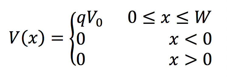
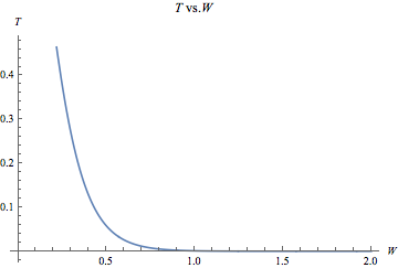 Fig. 3: This graph was produced in Mathematica using rough estimates for the energy values in the T equation. The numbers on the axes are not intended to represent actual quantities, and the graph merely suggests the shape of the function.
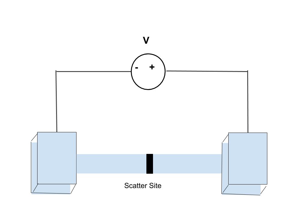


