Sarah Gittins and Lily Frye – Orbital Mechanics

Using the Euler cromer method, we will investigate the movement of solar entities in orbit. First, we will write a program that numerically finds the position and velocity of the earth as it orbits the sun. Second, we will write a program that numerically finds position and velocity of the moon as it orbits the earth as the earth orbits the sun. Third, we will write a program that numerically finds the position and velocity of a large star such as the sun as a massive planet orbits it, or rather as they orbit and affect each other. To calculate these movements we will use basic equations of motion and Kepler’s laws.

PHYS 375 – Project Proposal (Fall 2015)

My proposed project will address musical instrument modeling, namely for the instruments I play, the harpsichord and organ. Computational Physics, by Nicholas J. Giordano and Hisao Nakanishi, addresses the piano, among other instruments, in chapter 11, which will serve as a starting point for modeling other musical instruments that have their own unique physical characteristics. For example, the harpsichord plucks, rather than strikes, its strings, and modeling a more accurate plucking force along with other features of the instrument would form part of the project. Another example is the variety of sounds produced by the pipe organ due to different pipe materials and shapes. I intend to model at least one pipe type (more if the harpsichord part of the project proves too simple). In all cases, I intend to compare the “bridge force spectrum” (basically, the force waves of certain frequencies exert at the boundary) that I calculate to an actual signal from the instrument itself, which I will record and analyze. This will verify, or nullify, the models that I will build.

Alex Molina & Kadeem Nibbs Project Idea

For our project, we are interested in exploring realistic projectile motion as it pertains to the human body. While air resistance and spin often produce negligible effects for the objects in introductory mechanics, normally modeled as point particles, they can produce significant effects on objects with larger surface area and mass, such as the human body.

In addition to this, with athletic competitions often being decided by seconds in races or mere inches in jumping events, minimizing adverse effects can ensure victory. We are interested in modeling the human body in motion in MatLAB in Olympic jumping events, contorting limbs in obscure positions and seeing how it affects the ultimate outcome of the event.

Project Proposal: Applying Physics to Problems in Financial Markets

Many economists work on problems where they cannot be sure how different factors affect each other. In the context of physics, the Ising model is used to study the interactions between bodies that make up complex systems. A number of internal and external factors influence the way these bodies interact with each other to affect the whole system. There are several ways to solve Ising models, but one of the most pragmatic is the Monte Carlo method, which calculates the probability of certain factors occurring over and over again at varying probabilities until the system reaches an optimal level. Adam Warner and I would like study the ways these techniques aid problems done by economists. First, we will use MatLab to model a simple Ising system in the context of a physics problem relating either to magnetism or phase transition. From there, we will each look at different ways that Monte Carlo methods and Ising Models apply to financial models. This analysis will include a survey of utility-based decision making, market booms and crashes, and the volatility of stock pricing. We hope to compare the results we obtain through our MatLab programs to established studies done by financial institutions.

Audio Signal Processing

Audio signal processing is taking an audio recording, represented as a wave function of amplitude against time, and mathematically manipulating it, often in order to improve the quality.

Transposing the pitch of an audio recording is easy if you allow for changes in the length of the file. If you shorten the time of the wavefunction the frequency increases, and similarly if you lengthen the time of the audio file you decrease the frequency of the wavefunction. However, it is much more computationally intensive to transpose an audio file without changing its length. Fourier analysis is used to change the wavefunction from the time domain to the frequency domain, changing the frequencies represented, then using the inverse Fourier transform to return it to the time domain without lengthening the time of the file. You cannot simply linearly shift all of the frequencies represented in the Fourier transform because the harmonic ratios must remain intact.

This can be used for many reasons, entertainment being common, but there are scientific reasons as well; such as studying infrasonic and ultrasonic waves. The study of ultrasonic waves brings about some issues with computers. To capture ultrasound waves the sampling rate must be considered in order to avoid aliasing of frequencies above the nyquist frequency.

We are going to represent ultrasonic sound waves in the audible range.

by: Juan Vasquez & Robert Sciortino

Computational Physics Project Proposal

For my computational physics project I would like to investigate the relationship between the precession and the eccentricity of a planet’s orbit due to general relativity as detailed in chapter 4, section 3 of Computational Physics, by Nicholas J. Giordano and Hisao Nakanishi. Precession is the phenomenon of the rotation of the orientation of axes of a planet’s (elliptical) orbit with respect to time caused by the gravitational forces exerted by other planets. However, general relativity predicts deviations from the inverse-square law, which (for example) allows the Sun to contribute an additional 43 arcseconds per century to the precession of Mercury (as the distance between the two is small enough for the deviations to have an effect). The rate of precession examined in this project will only be that which is caused by the model planet’s host star. This will entail the construction of a planetary motion program using Newton’s law of gravitation and the Euler-Chromer method; which will later be adjusted to allow for the addition of a variable precession rate. The value of the planet’s perihelion will be held constant at the value for Mercury’s perihelion, but the eccentricity and size of the orbits will be allowed to vary. Mass of the planet will be held constant, at the same value as for Mercury.
If I have additional time left over I could also add another planet (such as Jupiter) to my code to make a three-body simulation of the “Mercury-like” planet.

Sushant Mahat and Mohammed Abdelaziz – PHYS 375 Project Proposal

Our project will be aimed at studying the behavior of a sample of N molecules when they are heated by a pulsed laser source. For this project, we will be using Newton’s second law, statistical mechanics, and the information on molecular dynamics simulations in Chapter 9 of Giordano and Nakanishi’s Computational Physics.

In our project we will tackle molecular heating simulations at different levels of difficulty. We will start simply by simulating gas molecules in a box and move on to more complex topics that involve heating and then finally pulsed heating of the gases. From these simulations we will study how long it will take for the gas particles to come to thermal equilibrium and how the speed distributions of the gas particles look when the system is in equilibrium.

After gases, we will try to create similar simulations to study the properties of crystalline solids. If we have time, we will also study the Fermi-Pasta-Ulam problem.
We decided upon this project as this is closely related to what we are studying in our thermal physics class right now and what we studied in classical mechanics in the past. Both branches of science are interesting and very challenging and we hope that undertaking this project will give us a better understanding of the concepts we have learnt so far.

Conclusion

Experimental vs. Theoretical Values

It was immediately apparent when I began collecting data for this experiment that the equations I derived to anticipate voltage and frequency values were not entirely accurate. Here I will calculate expected curve shapes and expected values of frequency and decay, and and compare them to experimentally measured values. The majority of the difference in theoretical vs measured data is the fact that there is some resistance in the circuit. It may be possible to discover this resistance from the future tests, if not from the current data.

Shape Of Potential Curve

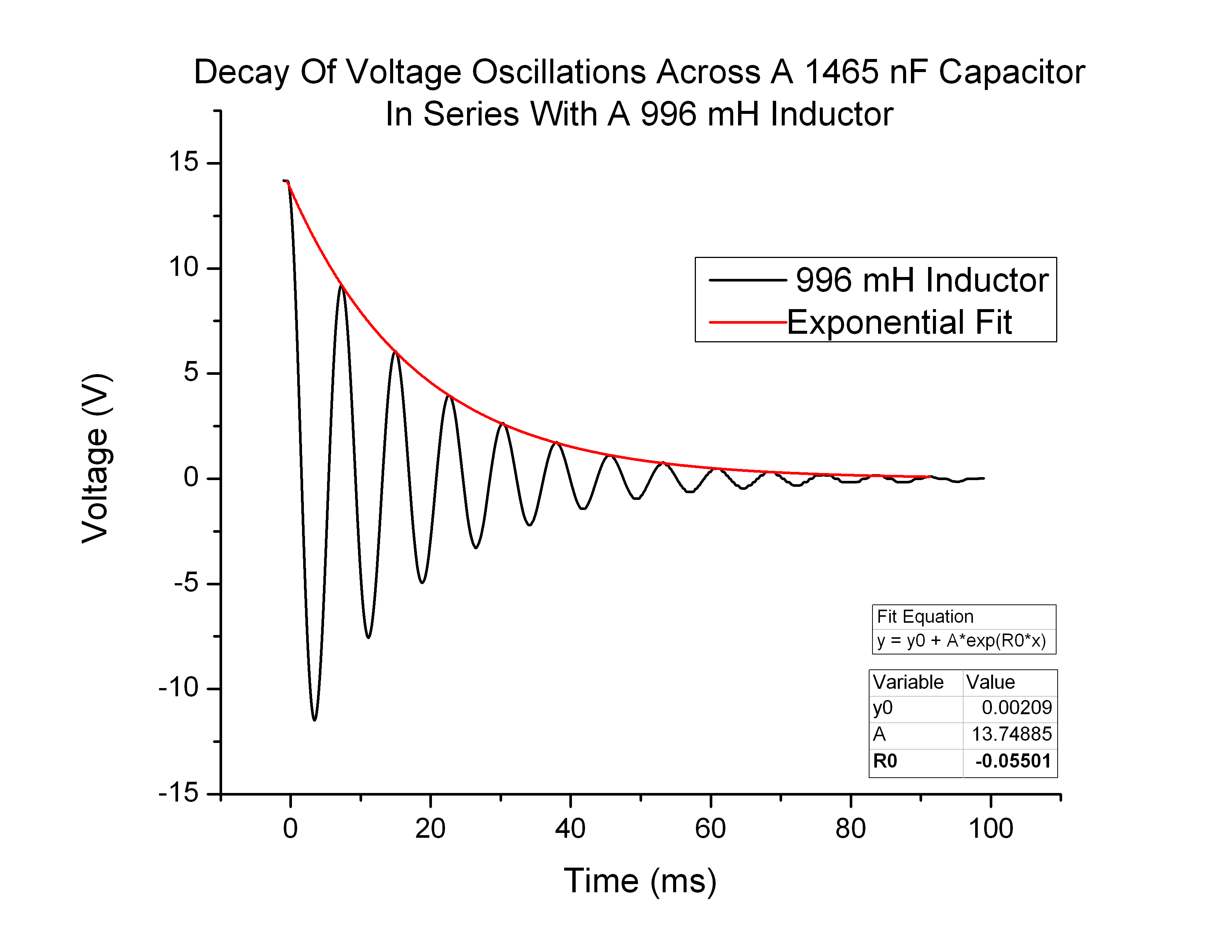
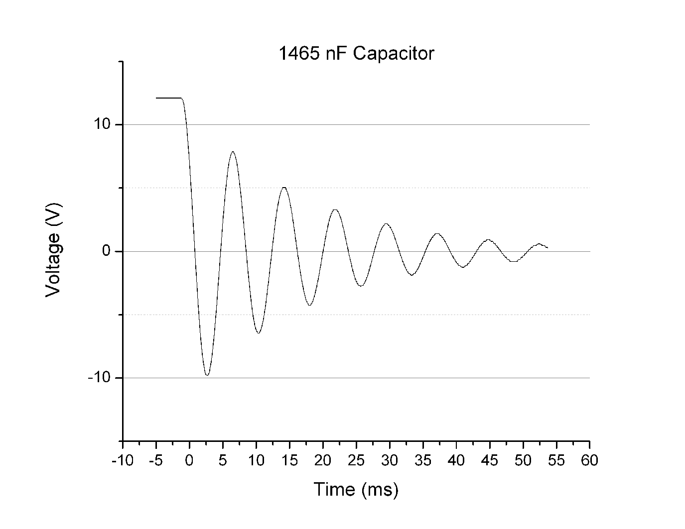
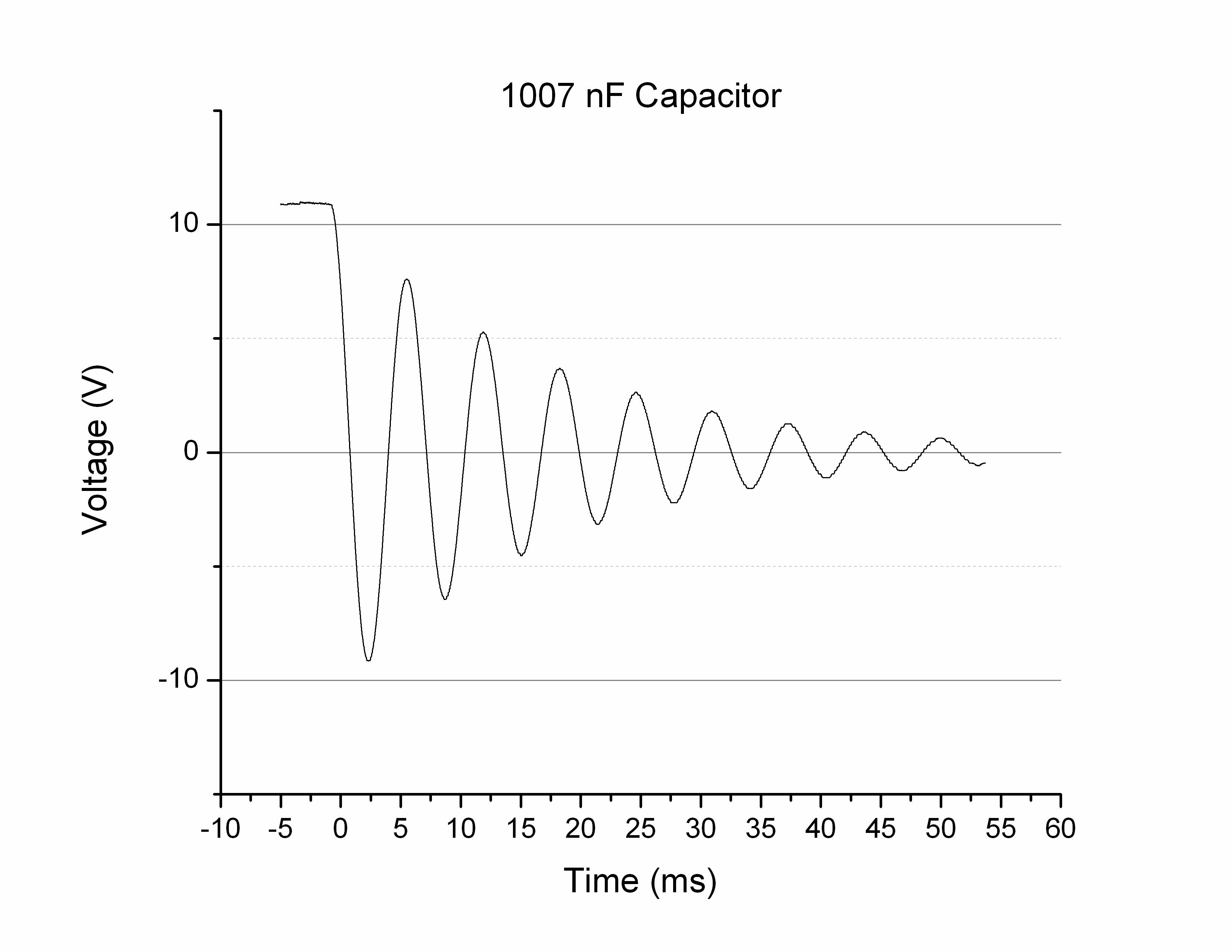
Figure 1. 1465 nF Capacitor and 996 mH Inductor in series.

In theory, the circuit I constructed was a LC circuit. This means there was no resistor in series with the capacitor and inductor components, and that the wires have negligible resistance. Theoretically the oscillations of the voltage after the capacitor discharged through the inductor should continue indefinitely. This is analogous to how an object on a spring would oscillate forever without drag/friction forces acting upon it. That being said, it is readily apparent that the oscillations did not continue indefinitely. In fact they took around a 10th of a second to dissipate (in the case of the 1465 nF capacitor and 996 mH inductor circuit above). This means that there is damping occurring on the oscillations. So while theoretically I built an LC circuit, experimentally it behaved more like a damped LC circuit, or an RLC circuit, as if there was a resistor in series with the capacitor and inductor. This means that the relevant governing equation was not $V\left( t\right)=V_{0}sin \left( \omega _{0}t-\delta \right)\left$ , but rather $V\left( t\right) =V_{0}e^{-\beta t}\sin \left( \omega _{1}t-\delta \right)$ . 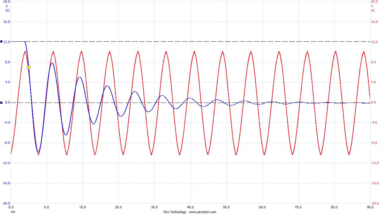Below (Figure 2) is the demonstration of expected shape (red) and measured shape (blue) of the voltage curve vs time as seen in my “Preliminary Data” post:

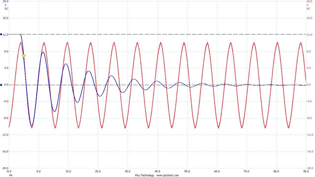
Figure 2

Frequency

To review,

$f = \frac{\omega}{2\pi}$ (1)

In Simple Harmonic Motion

$f = \frac{\omega_{0}}{2\pi}$ ; $\omega_{0}=\frac{1}{\sqrt{LC}}$ . (2)

But as we just discussed, because the circuit is not ideal and has an equivalent resistance, these oscillations are actually described by Damped SHM, the equations being as follows:

$V\left( t\right) =V_{0}e^{-\beta t}\sin \left( \omega _{1}t-\delta \right)$ (3)

$\omega _{1}\equiv \sqrt {\omega _{0}^{2}-\beta ^{2}}$ $\beta \equiv \frac{R}{2L}$ (4)

Thus

$f= \frac{\sqrt{\frac{1}{LC} - (\frac{R}{2L})^2}}{2\pi}$ (5)

Where, solving for R, we can estimate the equivalent resistance of the circuit:

$R=\sqrt{\frac{4L}{C}-(4 \pi L f)^2}$ (6)

Below is a table of values (Figure 3). On the left are all of the the experimentally measured values from this project. The expected theoretical frequency was calculated using Equation (2). The resistance of the circuit was estimated using Equation (6).

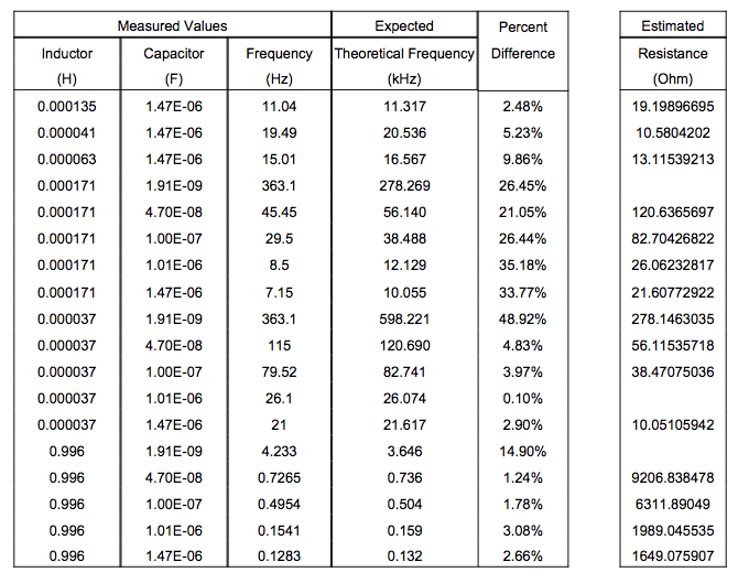
Figure 3

While the measured frequencies are not always very close to the predicted value, they are all well within an order of magnitude of each other, meaning the relationship defined by Equation (2) is clearly evident.

The estimated values of resistance, on the other hand, are extremely improbable. The resistivity of small connection wires is on the order of 10^-2 Ohms or lower. This indicates either a mistake in my derivation of resistance as a function of capacitance, inductance, and frequency, or a relationship that I don’t quite understand. It is possible that the equivalent resistance of the circuit changes as a function of voltage, or the change in current, in a way I do not know about.

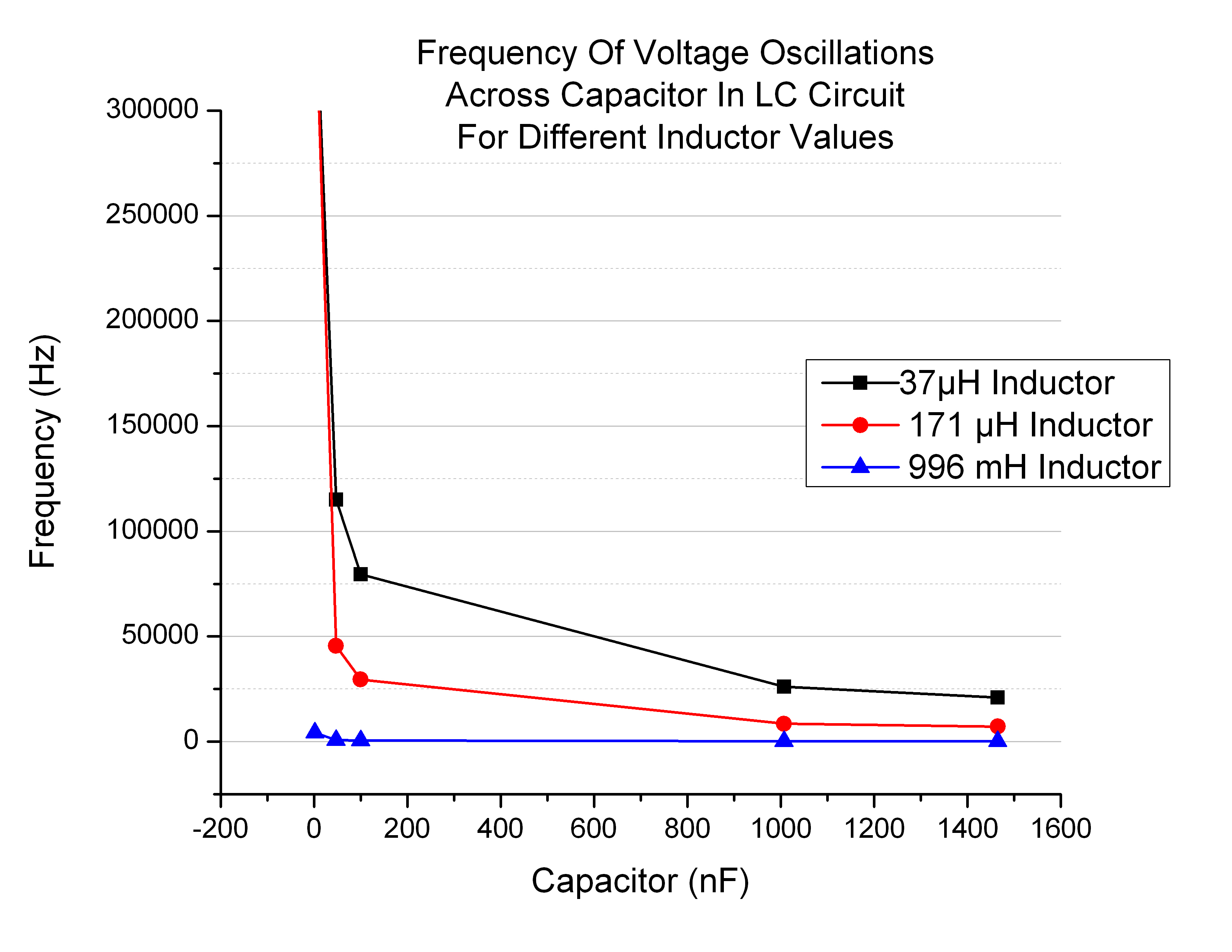
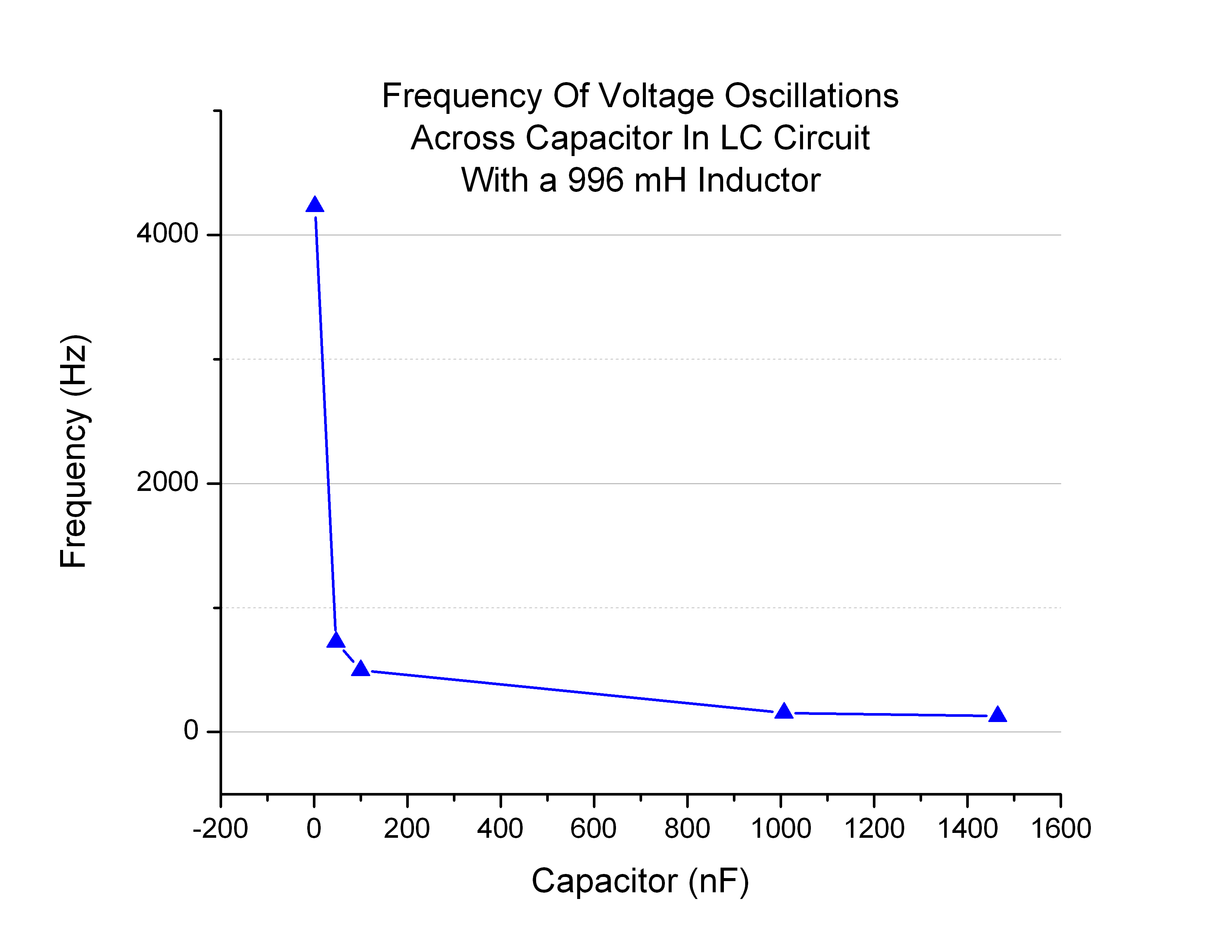
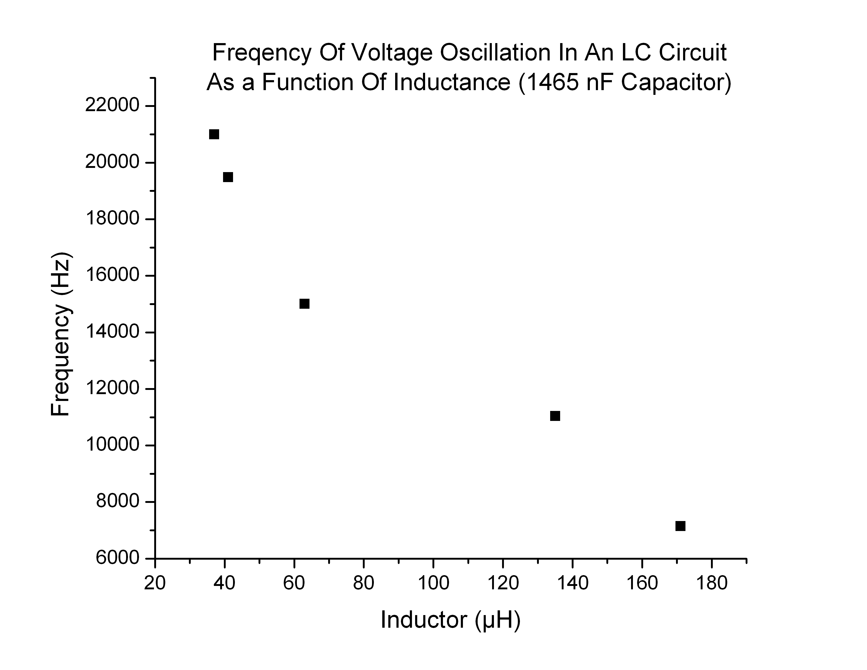
Overall, the graphs of frequency as a function of L or C (Figure 4) were the correct shape.

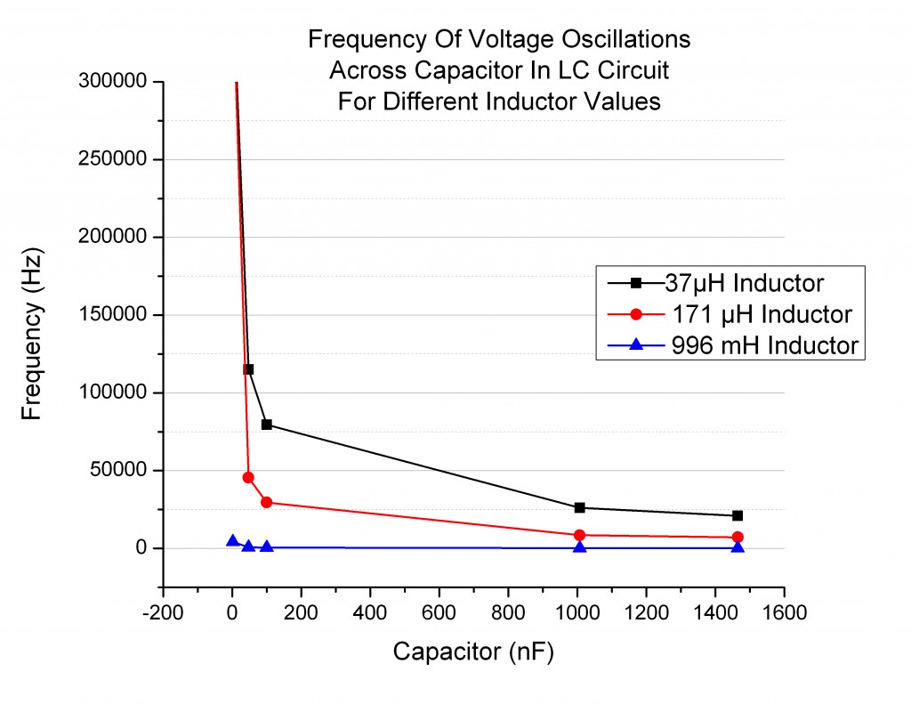
Figure 4

They reflect the predicted behavior of a $\frac{1}{\sqrt{x}}$ relationship, whose plot looks very similar (Figure 5). In our case the actual relationship is $f = \frac{1}{2 \pi \sqrt{x}}$ .

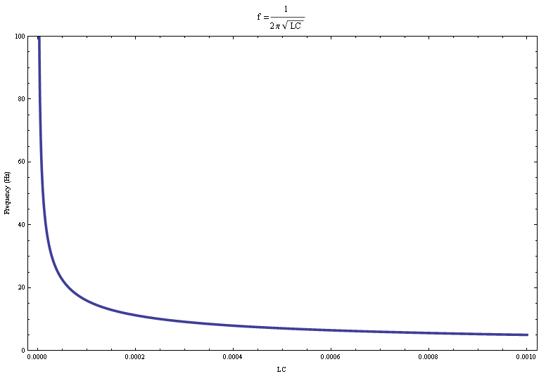
Figure 5 (Mathematica workbook: https://vspace.vassar.edu/mabjornsson/1%20over%20sqrt%20x.nb )

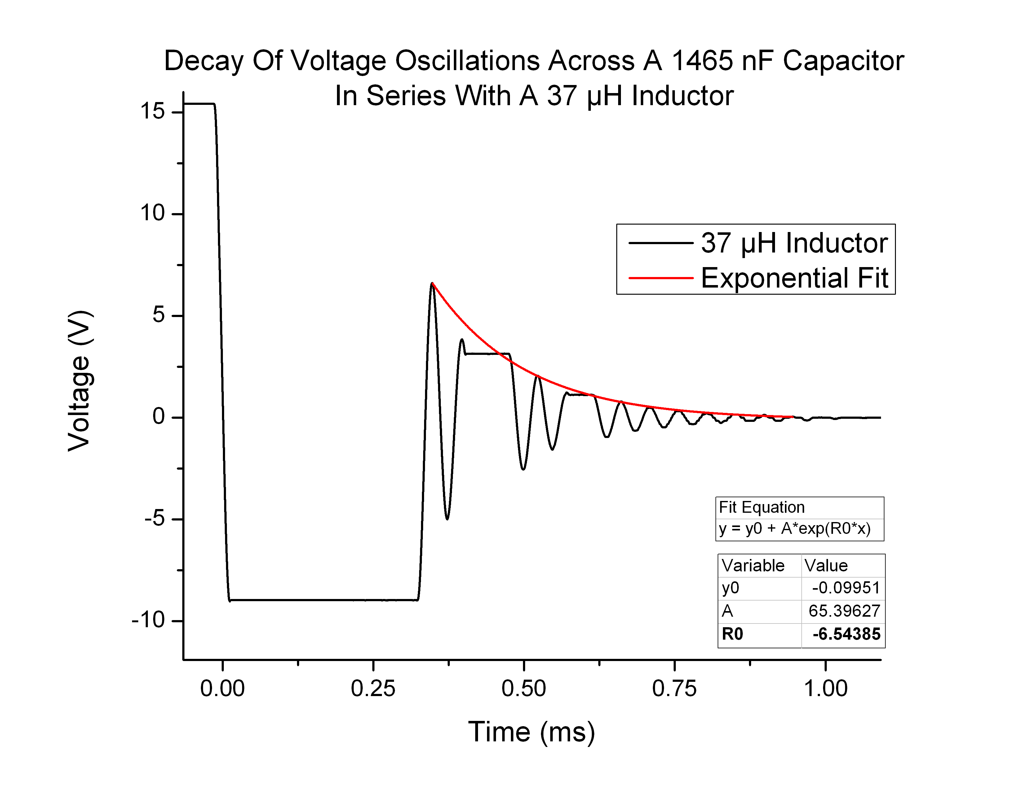
Exponential Decay and Circuit Resistance

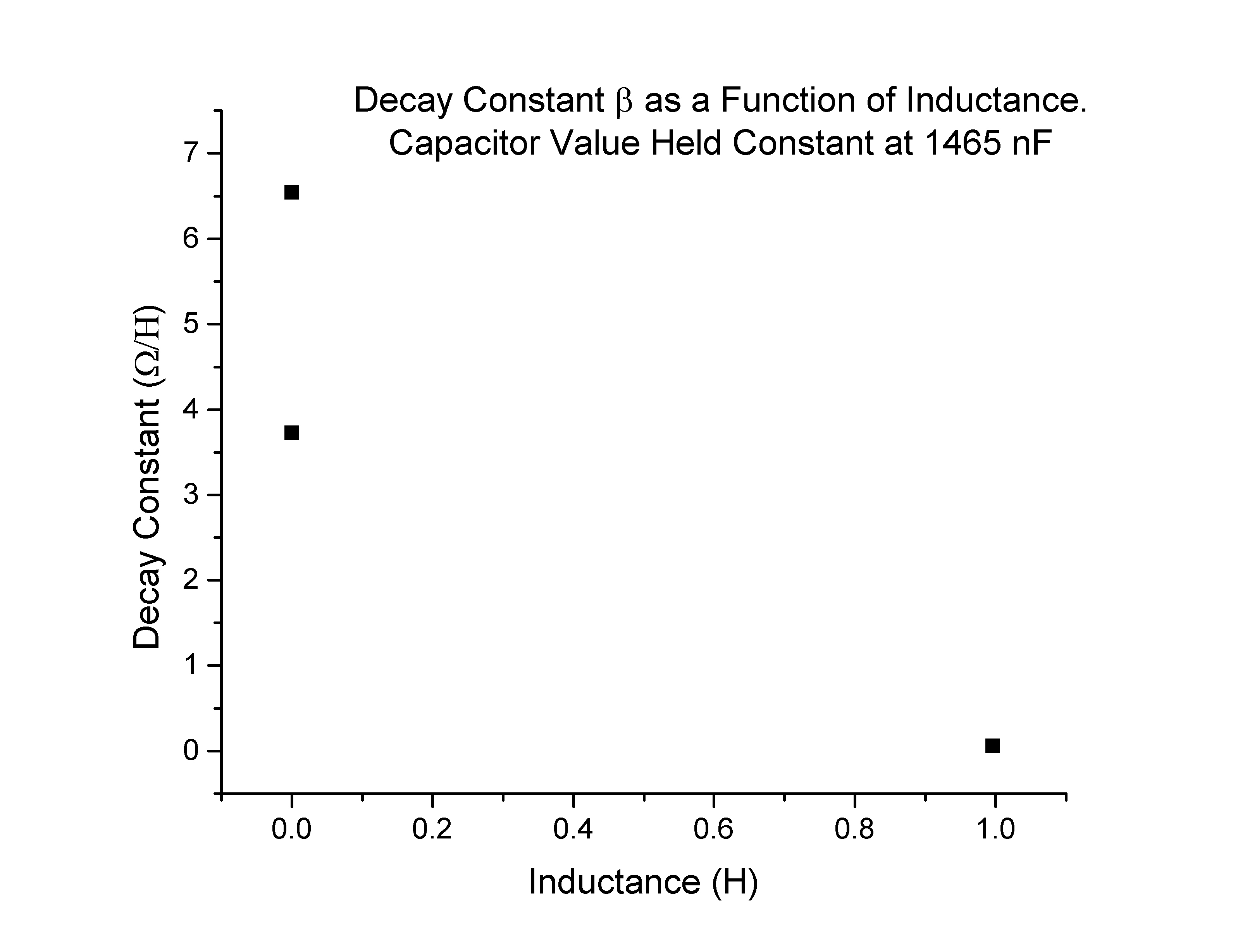
When the experimentally measured decay coefficient β is plotted as a function of inductance, the data points are sparse, and one should be cautious of drawing too many conclusions. That being said, the points I collected (Figure 6) do seem to match the expected values (Figure 7):

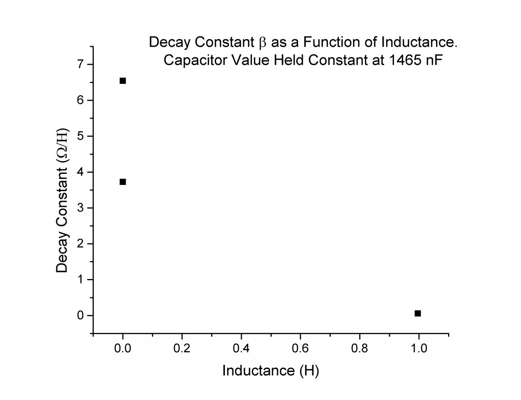
Figure 6

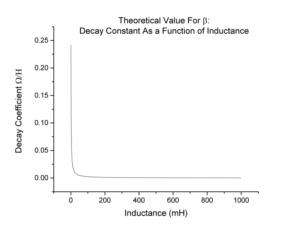
Figure 7

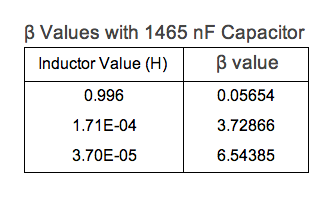
Finding Resistance Using β

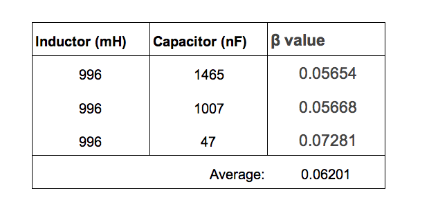
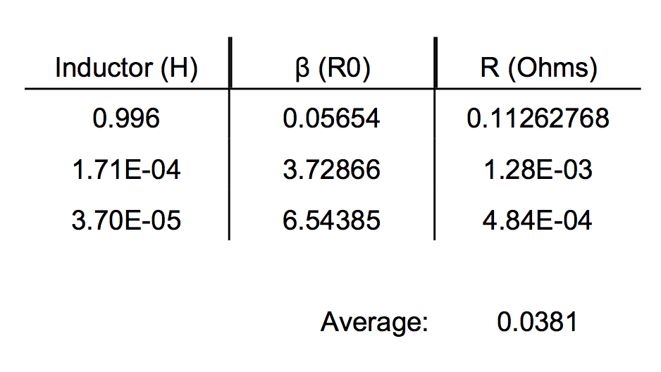
The decay coefficient β is related to L and R. Thus, since we know β and L experimentally, it should be fairly straightforward to calculate R empirically. In theory the resistance of the circuit should be the same for each measurement of β and L. Below is a table of measured values of β and L (Figure 8):

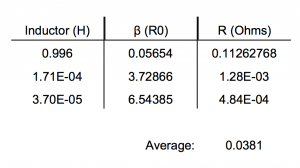
Figure 8

A value of 0.0381 Ω is a reasonable order of magnitude for a circuit with theoretically no inherent resistance. This order of magnitude is also large enough to be largely responsible for the decay of the voltage function across the capacitor.

Can Significant Conclusions Be Drawn From This Data?

With scatter plots with only three data points, the answer is “no.” To confidently confirm that my data was following anticipated trends I would need many, many more points. The most conclusive and illuminating data that I did generate wast the Voltage vs. Time graphs. These graphs were supposed to be undamped sinusoidal waves, but instead exhibited very clear damped oscillation. The collection of these curves was easy to repeat and allowed me to generate very reliable curves. These graphs confirmed that there must indeed be a significant equivalent resistance in the circuit to damp the oscillations.

Applications Of Findings

This experiment could potentially be an effective way to anticipate the inherent resistance of a circuit. My first method of using L, C, and f to find the resistance, clearly did not work, but finding the decay coefficient and from there calculating R, could very well be effective. From my limited data I got a reasonable solution, but would have to generate far more data points to confirm this resistance. It would be particularly interesting to use this method in an instructional lab if there was some way to actually measure the resistance of the circuit (maybe known values of wire resistivity, or a very sensitive meter). It would provide students with data analysis experience, such as fitting curves and using Origin Pro, as well as having hands on experience with damped harmonic systems.

Changes To Experiment

The biggest change I would make to this experiment would be to have a far greater array of capacitors and inductors at my disposal. I did not have enough to produce satisfying data. One problem I kept running into when collecting data was that one of my inductors was several orders of magnitude bigger than the others. It could have been handy to have just made my own inductors out of coils of wire. This way I would be able to change the inductance at will. Ideally I would also exchange many capacitors for one variable capacitor. It would streamline the data collection and allow for more methodical, precise data collection. I would also use components and measurement devices that could handle more than 15-20V due to the fact that such low voltage has a greater window for interference.

Sources Of Error

I have no idea how much my measuring devices and power source effect the overall resistance of the circuit. I also do not know if there are other sources of induction (albeit minor) within my circuit setup, either within components (such as the switch) or from the wires of my measurement tools coiling around themselves. There were many times when the discharge curve across the capacitor would take a strange shape that I can only attribute to some form of saturation, either the probe or capacitor. I do not know how this my have impacted my data.

Final Data

In this post I will present my actual data findings with minimal interpretation. In the next blog post, “Conclusion,” I will interpret the data I collected and compare it to expected values.

Preliminary Data Recap:

In my previous post I had measured the discharge of several different capacitor values in series with an inductor.

Below were the resulting plots of Voltage vs Time (Figures 1-3):

Figure 1

Figure 2

Figure 3

For the 1465, 1007, and 47 nF capacitors the measured frequency of oscillation was 128, 155, and 730 Hz, respectively.

Voltage As a Function Of Time and Frequency of Oscillation

It is helpful to layer these three plots on top of each other (Figure 4). In doing so we can readily compare the curves to each other.

Figure 4

From Figure 4 it is evident that the higher the capacitor value, the lower the frequency of oscillation. This is not surprising, given the equation that the frequency and inductor*capacitor product are inversely related: $\omega_{0} = \frac{1}{\sqrt{LC}}$ .

How are frequency and capacitance, or frequency and inductance related? I recorded the frequency of oscillation in several different LC circuits to try and illustrate this relationship. For three different inductor values I discharged five different capacitor values. The resulting plot (Figure 5) is below:

Figure 5

Because it is harder to see the shape of the blue line in Figure 5, I plotted it separately (Figure 6):

Figure 6

Figures 5 and 6 experimentally illustrate the inverse square root relationship between frequency and capacitance/inductance.

I then plotted the frequency of oscillation with respect to inductor value (Figure 7):

Figure 7

Exponential Rate Of Decay

If you take a look at Figure 4 again, notice that despite changing capacitor values, the exponential decay of each curve is relatively the same. The decay for each curve is the same because the decay coefficient β is a function of resistance and inductance, not capacitance( $\beta\equiv \frac{R}{2L}$ ). In Equation (1) you can see the decay term of the voltage, e^(-βt):

$V(t)=V_0e^{-\beta t}cos(\omega_1t-\delta)$ (1)

In order to measure the decay constant I used Origin Pro to fit an exponential curve to the peaks of the voltage plots. The formula used for this function fit was as follows:

Where R0 is the decay coefficient, -β

Figure 8 below is an example of this function fit:

Figure 8

I fit an exponential function to the 996 mH and 1007 nF, 47 nF oscillations as well, resulting in the table below (Figure 9):

Figure 9

Theoretically the β value should be the same for all of them.

In order to explore how the decay coefficient β changes I needed to change the inductor values. Because the voltage curves were more manageable at greater LC values, I used the largest capacitor I had and varied the inductor value. The results were as follows (Figures 10-11):

Figure 10

Figure 11

The resulting decay coefficients are as follows (Figure 12):

Figure 12

Which can also be represented in as a scatter plot, despite having so few points(Figure 13):

Figure 13

Critique: Modeling Electric and Magnetic Fields

At the end of the preliminary data section, the Electric Field of a bar electret is stated to be approximately that of two opposing charged point charges at either end of the bar. However, little explanation is given as to why the bar can be modeled that way. If there was a justification given for this model, such as modeling many charges arranged in a line to show that the net fields cancel aside from the two charges at either end, the data would significantly benefit from this. Finally, it is unclear in the final data whether or not you are modeling a bar electret or an electric dipole.

Additionally, it is unclear why you chose the specifications for the dipole bar magnet, as well as the surrounding constants and values for the other scenarios. Although it is clear from a knowledgeable individual’s standpoint why the charges were assigned the equations as they were, a layperson may not be able to interpret the equations correctly. Additionally, including the full derivations for each scenario on the preliminary data in mathematica would streamline the analysis of the data significantly, as the constants themselves would become more clear with this. Additionally, the equations that yield the specific graphs in the final data you are showing should be wrote, so that I we can associate the data and figures easily.

Finally, I suggest making the equations and derivations slightly more robust. By that I mean carrying out the derivations for these geometries in matter, as to better replicate the situations which a student may come across. Currently, this issue is approached without giving thought to the effects of polarization and the various materials involved. This may prove to both improve the depth and breadth of the project. Another concern that I have, although it may be a fault with mathematica, is that the field of the electret, does not show the field’s shape clearly. I suggest using a different graphing method, perhaps a contour graph, which would allow the interpretation of field lines much more intuitively. As such we would then expect the graph to take the shape of an imperfect dipole, as stated in your data.

Modeling and Experimental Tools with Prof. Magnes

Ideal for getting ideas and feedback on upper level physics tools.