Fundamental Rovibrational Spectrum of CO

Motivations

Protoplanetary disks are regions of planet formation around young stellar objects. Astronomers observe these regions to get snapshots of the planet formation process. Protoplanetary disks are optically thick at visible wavelengths, meaning that photons in the visible part of the electromagnetic spectrum from the star are absorbed by the disk and do not reach observers on Earth.  Millimeter wavelength light is not absorbed by the disk as much, and so by observing light in that range, astronomers can learn about the morphology of disks. One key molecule abundant in protoplanetary disks is carbon monoxide (CO). Because of the low temperatures of disks (around 40 K), the energy transitions observed fall in the rotational and vibrational (rovibrational) regime.

Overview

When two atoms form a stable covalent bond, they can be thought of semi-classically as a two atoms connected by a spring. That spring can vibrate, and the energies of the vibrations can be found by treating the bond as a harmonic oscillator. This gives us
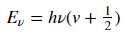
,

where v is the vibrational quantum number associated with different vibrational energy levels.

Diatomic molecules can also rotate in different ways, corresponding to different rotational energy levels. Assume that the molecules act as rigid rotors, meaning you assume that the molecules are connected by a solid rod as they rotate so that the bond length does not change. This lets you solve the Schrödinger equation and get the allowed energies.The energy associated with a rotational state is given as

,

where j is the rotational quantum number and I is the moment of inertia of the molecule. Molecular spectroscopists define the rotational constant B

which has  which as units of energy. B changes based on the molecule, and for CO I found the value of B to be as listed above.

My goal with this project was to explore the fundamental rovibrational spectrum of CO. I first investigated energy in a rovibrational system and plotted how it changes for different rotational states. I did this using Python 3 and the libraries NumPy and Matplotlib. Then I modeled the intensity of different lines in the fundamental spectrum of CO and overlaid it with experimental data taken from the high-resolution molecular absorption database (HITRAN).

Selection Rules

Selection rules describe what quantum state transitions are allowed in a given system. The fundamental spectrum in this context refers to the transition in which the vibrational state (v) changes by +- 1. This gives rise to the selection rules. If the vibrational state changes by +- 1, the rotational state must also change by +- 1, no more and no less. In this field, the [forbidden] transition of Δv = +- 1 and Δj = 0 is called the “Q branch”, and it appears in Fig. 3 as an empty spot in the middle. When the rotational state changes by +1, the transition is said to be in the “R branch”, and when it changes by -1 the transition is in the “P branch”. These selection rules can be summarized as:

  1. Both the vibrational and rotational quantum numbers must change
  2. Energy of rotation can be added to (in the R branch) or subtracted from (in the P branch)

The energy of transitions in the R and P branches respectively are:

where the first term corresponds to initial energy of the system before the transition.

Though the energy of rotational states increases with increasing j, the difference between two consecutive levels is always 2B, where B is the rotational constant. This can be seen in Fig. 2. If going to a higher rotational state (in the R branch), add 2B to get the new energy level; subtract 2B for a lower state.

Results

Energy of rotational states

Fig. 1

Fig. 1 shows how rotational states increase in energy based on the equation listed above. Despite the slope of this graph not being constant, a look at the change in energy between levels reveals an interesting fact about rotational transitions.
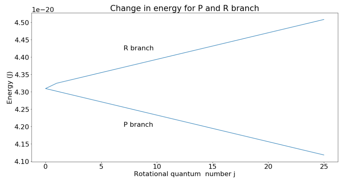
A constant slope means changes in energy are equal

Fig. 2

Fig. 2 plots change in energy vs. rotational quantum number for the R and P branches. The Q branch is the corner point where no transitions occur. From the graph, we can see that if undergoing a transition on the R branch, the energy of the state will increase linearly from one state to the next. That change is given by the slope of the graph which was found to be 2B, as expected. Similarly, the P branch energy transitions decrease by 2B from one transition to the next. Note that the rotational quantum number j can only increase or decrease by 1 with each transition.
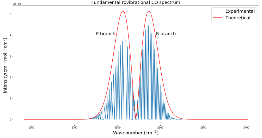
Theoretical and experimental rovibrational CO

Fig. 3

Fig. 3 plots the theoretical relative intensities of different transitions based on the following equation:

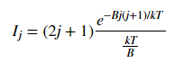
where k is the Boltzmann constant and the temperature T was set to 300 K. The blue spectral lines come from experimental data from HITRAN. The x axis is given in wavenumbers, a unit commonly used in molecular spectroscopy.

Discussion

Fig. 3 was the most challenging result for me to produce and took several weeks of trying many different methods. Plotting the actual data was somewhat simple with Python, but calculating the relative intensities took me down many dead ends before finally getting the end result. Different sources listed different equations for intensity and different values of B. Eventually after calculating my own B and using an equation from Bernath, I was able to get the desired result.

I expected that the theoretical and experimental distributions would not match exactly, and that is because real molecules do not act exactly like rigid rotors. They experience centrifugal distortion and rovibrational coupling, which both add complications to the simplistic energy equations I used. However, my goal was to calculate the simplistic version of the fundamental rovibrational spectrum, and I accomplished that. In future work I would like to try to add complications to the model to better fit real data. I would also like to see how the environment of a protoplanetary disk could affect the spectrum.

References

Spectrum of Atoms and Molecules by Peter F. Bernath

Fundamentals of Molecular Spectroscopy by C. N. Banwell

Chemistry LibreTexts

SpectralCalc

HITRAN

Observing Quantum Entanglement Through Spontaneous Parametric Downconversion

In this project, I (and partner Jay Chittidi) investigate the concept of quantum entanglement in an experimental context. I will show how entanglement not only relates to the concept of superposition but also how it furthers our understanding of the differences between the laws of Quantum Mechanics and Classical Physics.

What is Quantum Entanglement?

Entangled particles are in a special kind of superposition of states such that either of their wavefunctions cannot be considered independently from the other. In other words, a measurement on one of the particles instantly affects that of the other.

To illustrate how an entangled state differs from a simple superposition of two states, we can consider two photons that have two corresponding polarization states, horizontal or vertical. A non-entangled state for each photon would look like the following:

[1]

In this case, each photon is in a superposition of vertical and horizontal polarization and the coefficients A,B,C, and D represent the probability of measuring vertical or horizontal for each photon.

If the photons were in an entangled state, their wavefunctions could look something like this:

[2]

In this case, both the photons have the same wavefunction, which depends on the horizontal/vertical polarization state of either photon. This means that any measurement of one photon will depend on the measurement of the other. Note that there are multiple ways to achieve this; the equation above is just one example.

To illustrate this further, we can calculate the expectation value of some measurement, by assuming there exists some hermitian operator, O, for this measurement:

If the photons were not entangled:

[3]

If the photons were entangled,

[4]

Equation 3 shows that the non-entangled photon has an expectation value for the measurement that only depends on its own polarization state. In contrast, equation 4 shows that this expectation value for an entangled particle depends on the polarization states of both particles. Thus, at the time of the measurement, both particles will instantaneously collapse into corresponding states.

Hidden Variable Theory

We can also examine entanglement through the lens of hidden variable theory. As stated above, when one measurement is taken from a member of an entangled pair, the other one instantaneously collapses into a corresponding state based on their mutually dependent wavefunction. Even if the photons are on opposite ends of the universe, this collapsing effect would theoretically be the same. If the wavefunctions collapse instantaneously even at astronomical distances, then information needs to travel faster than the speed of light. One explanation for this “magical” phenomenon is that there exist hidden variables that predetermine the outcome of each measurement before it occurs.

In 1969, Clauser, Horne, Shimony, and Hotle (CHSH) created a generalized hidden variable theory which they used to derive an inequality that would only be true if hidden variables are at play in a given measurement. [2] They did this by assuming the outcome of a given measurement depends on the independent parameters involved and some arbitrary “hidden variable” in some way. Then, they derive an expression, Bell’s inequality, which will always be true for a given set of measurements if hidden variables are involved. The derivation of this inequality is not trivial and purely mathematical, so it is not relevant to this project. They also proposed an experiment to test their inequality that consists of measuring the number of coincident photons as a function of polarization of either photon. If we can prove that no hidden variables exist, then we will show that the behavior of entangled particles contradicts our understanding of classical physics.

Testing Quantum Entanglement Experimentally

To conduct our entanglement experiment, we utilized the phenomenon of spontaneous parametric down-conversion (SPDC). SPDC occurs when light passes through a nonlinear crystal (in our case BBO). A small number of photons that pass through the crystal split into two photons with equal energy that is half that of the incoming photons. They also have the same polarization that is orthogonal to the polarization of the incident photon due to conservation of angular momentum.  In our experiment, we sent a purple laser first through a half-wave plate to polarize the laser light at 45 degrees. The polarized laser light then passed through two BBO crystals oriented perpendicular to each other. This means that the down-converted photons could either be horizontally or vertically polarized, but since we can’t predict which crystal produced the pair, we don’t know their polarization. This phenomenon causes the photons to be in an entangled state, where the measured polarization of one photon depends on that of the other.  If the photons were not entangled, they would be in a randomly mixed state of horizontal and vertical polarization, whereas entangled photon pairs would have correlated polarizations.

The following formulas define variables, E and S, which don’t have a physical meaning. These formulas are just CSHC’s original hidden variable theory rearranged in a more convenient manner.[1][3]

[5]

 [6]

In these formulas, N is the number of coincidences recorded for the given combination of polarizer angles. Theta1 and theta1 prime are any two polarization and angles for detector A and theta2 and theta2 prime are any two polarization angles for detector B. Based on the work of CHSH S ≤ 2 if hidden variables are involved in the measurement of coincidences.[1][3] Thus, the expected results of our experiment would be an S that is greater than 2.

Experimental Procedure

Figures 1 and 2 show our experimental setup. The laser is shot through the half-wave plate, the BBO crystals, and also a quartz that corrects for the phase shift of the laser light.

We can see that the two detectors on the other side of the optical table are approximately equidistant from the principle beam in order to detect the two streams of down-converted photons. There is a polarizer in front of each detector in order for us to test the CHSH hidden variable theory. We also placed infrared filters in front of each detector so that they would only detect the stream of infrared photons.

Figure 1: Birds-eye view of experimental setup

Figure 1: Close up of detectors with polarizers in front

We used a LabView program (made by previous Vassar students) to record the total number of coincidences in each a 10 second interval. A coincidence is recorded every time the detectors register a photon instantaneously. Since the down-converted photons are in an entangled polarization state and have correlated polarization, the number of coincidences is a function of polarizer angle. The number of coincidences is also the measurement needed to verify equations 5 and 6.

Since S depends on configurations independent calculation of E, and each calculation of E depends on the number of coincidences at four polarizer configurations, we needed to measure the number of coincidences at 16 polarizer configurations in total.

Results and Conclusions

Table 1 shows the results of our experiment. The number of coincidences is clearly a function of polarizer angle, which indicates that the photons are in fact in an entangled state.

Table 1: Coincidence counts and total counts in each detector at each of the 16 combinations of polarizer angles. The first two columns show the angle of each polarizer. The third column shows the counts in detector A, the fourth shows the counts in detector B, and the fifth shows the coincidence counts.

Our final value of S, using equations 5 and 6 was -0.0465±0.0396. Unfortunately, this obeys Bell’s inequality for hidden variables, which is the opposite of what we had expected. We know from many previous repetitions of this experiment at other institutions, that Bell’s inequality should not hold in this experiment.[1][3] The uncertainty in our value of S is also about the same as the calculated value itself, so we are not very confident in our result.

There are various sources of error that could have resulted in the data we collected. There could have been some sort of light pollution that we weren’t accounting for or some hardware error. However, since our experimental setup has been extensively tested by previous students, these effects probably weren’t significant enough for us to get such an inaccurate value of S.

The most likely cause of the discrepancy between our data and the CHSH theory is improper alignment. Most of our time working on this project was spent attempting to align the laser. We struggled not only to align the detector with the beam infrared photons, but also to maximize the coincidences. For a more detailed description of our struggles, see Jay’s project.

From comparing our data to the data collected by Dehlinger and Mitchell using a similar experimental setup[1], we have deduced that at a given polarizer angle for detector A, the number of coincidences should vary sinusoidally with the polarizer angle for detector B. Figure 3 shows that at the different values of angle for polarizer A, the number of coincidences does not vary in this fashion with the angle for polarizer B.  We think that we could solve this issue by aligning the two detectors more thoroughly. The down-converted photons are actually emitted in ring, where photons across from each other are entangled pairs (illustrated in Figure 4). This means that if our detectors weren’t on the exact spots on the ring that correspond to an entangled pair, our data would not necessarily be consistent with CHSH theory or previous results. For future research, if we were able to place both detectors in some sort of circular mount with adjustable positions, then we would be able to more easily identify these exact positions. We also began our experiment with detector A already aligned and proceeded to align detector B. It is possible that we would have needed to align detector A more exactly in order to locate the correct ring positions.

Figure 4: Number of coincidences as a function of polarizer angle for detector B (beta) at different values of polarizer angle for detector A (alpha).


Figure 5: Schematic of SPDC. The entangled pairs are emitted in all orientations but at the same angle. They end up emerging from the BBO crystal in a ring shape, with entangled pairs exactly across from each other.

Regardless of some clear experimental issues, we were able to observe quantum entanglement in action. Although the number of coincidences we recorded did not show the correct dependance on polarizer angle, they displayed a clear relationship. This is a clear indicator that when one member of an entangled pair is counted, the other must instantaneously collapse into a corresponding polarization state to be counted by the other detector. And although we did not end up disproving CHSH’s hidden variable theory, our calculation of S came with an unreasonable uncertainty, so our results cannot prove that hidden variables exist. Inconclusive results aside, this project was very useful in illustrating the concepts of quantum entanglement and hidden variables, which relate to the most fundamental concepts of quantum mechanics such as superposition and deviation from classical mechanics. If anything, this experiment allows us to observe the oddity of quantum mechanics by simply counting photons.

References

[1] Dehlinger, Dietrich and Mitchell, M.W. “Entangled photons, nonlocality and Bell inequalities in the undergraduate laboratory.” American Journal of Physics 70, 903 (2002).

[2] John F. Clauser, Michael A. Horne, Abner Shimony, and Richard A. Holt. “Proposed Experiment to Test Local Hidden-Variable Theories” Physics Review Letters 23, 880 (1969).

[3] Galvez, Enrique J. “Correlated Photon Experiments for Undergraduate Labs” Colgate University (2010).

Escape the Potential: A Board Game Approach to Teaching High School Students

Title image of Escape the Potential

What We Made

Escape the Potential is a card game focused on teaching high school and early college physics students about concepts from quantum mechanics. More specifically, the game is focused on presenting students with an introduction to the many mathematical concepts that come up in quantum mechanics as well as some of the more recent technological achievements related to quantum mechanics. This Rule Book outlines the basic rules of the game. Additionally, there is an additional card appendix  that is included in the game. The card appendix has a short paragraph descriptor of each concept listed on the cards. Below are images of the cards and game boards which you can cut out in order to play the game. Maddy(see QM–>Maddy) and I worked on this project together, and she handled more of the pedagogical issues of how to best present information to the students playing the game. I focused on making the cards and writing out the rules of the game.


Outcome of Playing Escape the Potential

Students who play this game should come away with new knowledge about quantum mechanics after playing. While it is possible to play the game without learning the concepts underlying each card, the game exists as an educational tool, and this aspect of the game should be included when playing the game. We wanted the game to be an active learning process where the game encouraged students to learn about the theory of the cards without forcing it onto them. By including a card index in the game, we hope that the students familiarize themselves with the repetitive usage of the terms and concepts in the game. Here is a lesson plan for the game which can be provided for teachers so as to make the use of the game in the classroom as seamless as possible. See Maddy’s post for more information on the pedagogical goals of the game.

Playing the Game

While the rule book has all the rules that are needed for playing the game, here is a quick run down. Each player starts off with a deck containing 3 Blackbody Radiation cards and 2 Wavefunction cards. Each turn, players play cards trying to move up the eigenstates of the well(which correspond to the energy levels of the well) and earn Eigencoins for however high up the well they are. They can then buy cards to add to their deck to move higher up the well until the game ends when a player escapes or tunnels out(only applicable to finite wells).

In the gallery below are images of Mike (Thank you!) starting to play the game. While not pictured, there are students who were very helpful in providing us with feedback about the game. As a result of the play testing, we had changed several of the rules and tried to focus the game’s mechanics and change a few of the rules. If anyone wants to take a study break, the game is available to play in SP 201.1, where it is located on the top shelf of the book library.


Final Thoughts

I found the process of building Escape the Potential to be an incredibly rewarding experience. Not only did it force me to learn about the essence of each physics concept, but it also allowed me to be creative during a stressful time of the year.  Coming up with the concept of the game was a little difficult, as we knew we wanted to use cards and that we also wanted to come up with an original game, but weren’t exactly sure where to start. Spitballing ideas and playing other games was what took us to the current design of the game. Just as Escape the Potential does, the process of creating the game was itself an active learning process which allowed us to learn and understand quantum mechanics moreso than just reading a book about the concepts. Working with Maddy taught me a great deal about pedagogical goals when implementing a game that I would not have thought of by myself. By keeping the game educational, Maddy showed me why including certain topics are important and why some topics should be saved until the students have learned more about physics. Ultimately, we were able to come out of the project with a tangible game that can be kept and played in the future.


Acknowledgements

The game is modeled after the board game Dominion, which follows a very similar game progression, except another type of card, victory cards, is introduced into the game.

All images used in the game came from Wikimedia and fall under the Creative Commons Attribution 2.0 Generic License, which allows for noncommercial reuse of the images.


Viscous Drag and Motion

Overview

This project aimed to simulate the viscous drag forces that occur when a ball falls in fluids with different densities and viscosities, resulting in different Reynolds numbers. In this case, there are two graphs produced. The first shows the ball falling in the medium in phase-space. The second shows the vertical distance traveled by the ball in time. The  ball falling in the fluid with the larger Reynold number should take a  longer time to fall because the drag forces on the ball are greater. Fluids include both liquids and gases.

Reynolds numbers determine the type of flow the fluid will make. When Re<<1 the fluid follows Stoke’s Law. When Re>>1 the fluid does not,it follows the Navier-Stokes equations. The Reynolds number is a proportion of the inertial forces to the viscous forces, Re = inertial/viscous.

Motivations

While I studied abroad, I took a fluid dynamics class that covered the Navier-Stokes equations and complicated geometries of objects moving in fluids. The most basic geometry is a sphere in 3D and a circle/disk in 2D. I wanted to be able to visualize and create a code that could interpret various inputs for fluids and produce a 2D plot of the motion. It proved more difficult to do than initially thought because I do not have a solid background in fluid dynamics, just that one course. As a result, I referenced derivations for the Navier-Stokes, but most were more complicated than the 2D system I wanted to model. I referenced my notes from the course too and YouTube videos from MIT.

Figures (click on the images to make them larger)

water_vs_honey

Figure 1. The parameters of this plot are those of water and honey at room temperature (20° C). The viscosities are 1.0 (Pa s) and 1.36 (Pa s) and the densities are 0.7978 (kg/L) and 7.20 (kg/L) respectively. The ball travels slower in the honey, Re2.

randomvalues

Figure 2. The parameters for this plot are viscosities of 32 (Pa s)  and 400 (Pa s), densities of 20 (kg/L) and 75 (kg/L), and kinematic viscosities of 1.6 and 5.33, respectively. The Reynolds numbers are displayed on the plots. The ball moves slower in the larger Reynolds number fluid.

Fluid Mechanics Physics

screen-shot-2016-12-13-at-14-44-04

The above equations are the Navier-Stokes equations in 3D for cartesian coordinates. For the 2D version that I used, the z-direction components are removed. These equations are only used for when Re>>1, for high Reynolds numbers. Because the Navier-Stokes equations can only be solved for very specific cases I simplified the process by using the drag equation,

screen-shot-2016-12-13-at-14-45-17

and then solved Newton’s second law for the vertical and horizontal directions, and formulated the kinematics equations. Buoyancy forces were ignored. This is a different case than than when Re<<1.

When Re<<1, the system follows viscous drag using Stoke’s Law

screen-shot-2016-12-13-at-14-46-07

From here you can solve Newton’s second law and formulate the kinematic equations again. Stoke’s Law only works for these cases, otherwise Navier-Stokes and the drag equation are used. Buoyancy forces were ignored here too. 

Results

Computational fluid dynamics (CFD) is a growing and complicated field of both mathematics and physics. The program I developed is part of the general sphere of CFD but not close to the type of programs are used and developed. CFD is used to simulate airplane designs, model the way fluids flow around objects. My program has some bugs because of the simplifications I used for the equations. By using an adapted version of the Navier-Stokes equations, not all parameter values work correctly with the model. For the many combinations of inputs, however, the larger Reynolds number fluid produces a slower movement in the fluid.

Conclusion

In the future, I would like to fix the bugs caused by the simplifications and possibly create a program that uses the Navier-Stokes equation in its full 3D form. If possible, it would be useful to have a GUI for the program because that would allow the user to more easily see the differences in the motion when the viscosities and densities of the fluids are changed. Perhaps adding more than two fluids to the model as well as making the visualization as a movie and not stagnant plots.

References

http://soliton.ae.gatech.edu/labs/windtunl/classes/hispd/hispd06/ns_eqns.html

http://www.personal.psu.edu/wzl113/Lesson%20Plan.htm#GF

http://scienceworld.wolfram.com/physics/StokesVelocity.html

https://www.grc.nasa.gov/www/k-12/airplane/nseqs.html

https://www.grc.nasa.gov/www/k-12/airplane/reynolds.html

Analysis of C. Elegans Worm Diffraction Patterns using Lag, Density, and Poincaré plots

Overview & Background:

For my project, I analyzed non-saturated data taken in Professor Jenny Magnes’ laboratory of “roller” and “wildtype” C. elegans. worms. The goal was to use computational techniques to differentiate between worm types. To this end, I created three different types of graphs: lag, density, and Poincaré plots. All three used normalized data. Although my lag and Poincaré plot codes create 2D plots comparing non-lagged to lagged data as well as 3D plots that compare multiple lags, I am only including the 2D plots here due to the number of graphs I have.

Lag plots display the value of the data at time (t) versus the data at time (t – lag), where lag is a fixed time displacement. These plots determine whether data is random or not. They are one method for inferring information about dynamical attractors from observations.[1] The time delay is used to reconstruct the attractor. I plotted lag plots with lags of 200 and 400 (Figs. 1-2).

I then created density plots by binning the data into a 50 x 50 matrix and plotting the intensities of values in each bin (Fig. 3). These plots give information about the number of times point (x,y) appears in each plot by representing the counts with color. The density plot code also calculates the area of each plot divided by the area of values equal to zero (AreaRatio) and the area of each plot not equal to zero over the area of values that are (zeroRatio) (Fig. 5). These ratios describe the motion of the worms, specifically how much area they use to move around in.

Finally, I created Poincaré plots by plotting each value (point at t) against the next chosen value (point at t + lag) (See Fig. 4). Poincaré plots are return maps that can be used to help analyze data graphically. The shape of the plot describes how the system evolves over time and allows scientists to visualize the variability of their data.[2] They have two basic descriptors: SD1 and SD2.[3] Defining the “line of identity” as a 45-degree diagonal line across the plot, SD1 measures the dispersion of points perpendicular to the line of identity while SD2 measures the dispersion of points along the line. My code calculates and returns these statistical measures as well as the ratio SD1/SD2 for each lag determined by user input. For this project, I used lags of 1 and 100 (Fig. 6).

Results:

I. Lag Plots

Fig. 1 Lag plots of Roller Worms 3.20, 3.26, and 3.34 for lag values of 100, 200, and 400.

Fig. 2 Lag plots of Wildtype Worms 18, 19, and 26 for lag values of 100, 200, and 400.

 II. Density Plots

Fig. 3 Density Plots of Roller worms 3.20, 3.26, and 3.34 (left) compared to Wildtype Worms 18, 19, and 26 (right) with lag 200

III. Poincaré Plots


Fig. 4 Poincaré Plots of Roller Worms 3.20, 3.26, and 3.34 (top) and Wildtype Worms 18, 19, and 26 (bottom) for lag values of 1 and 100

IV. Data

Fig. 5 Values of SD1, SD2, Ratio of SD1/SD2, Area Ratios, and Zero Ratios for Roller Worms 3.20,3.26, 3.32 (left) and WildType Worms 18, 19, and 26 (right) for lag values of 100, 200, and 400 as well as average values per worm-type (bottom).

Discussion:

The lag plots indicate that my data is non-chaotic because they all had non-random structures. There appears to also be differences between worm-types, although this difference is difficult to quantize. As the lag increases, the lag plots appear more chaotic for both worm-types, moving from aligning with the x = y line to appearing more random and diffused. The plots show a difference between worm-types, but quantifying this difference will take further analysis. Wildtype worms tended to fall closer to the x = y line than roller worms. This is a sign of moderate autocorrelation. This suggests prediction of future behavior is possible using an autoregressive model.[4]

The density plots show a clear distinction between worm-type, with rollers tending to have more circular-shaped plots with highest intensity values at the center while wildtype worms appear to take up less of the plot area, with highest intensity values along the diagonal and at the center of the plot. This is confirmed by the area and zero ratios (Fig. 5). Wildtype ratios were on average larger than those of rollers, with area ratio values ranging from 0.04-0.4 more and zero ratio values ranging from 0.1-0.4 more for rollers. This gives us a quantifiable way to measure the difference between the motions of the two worm-types. However, whether these differences are statistically significant or not remains to be seen.

The Poincaré plots show little difference from the x = y line for a lag of one. However, at lag 100 they do deviate from the line. Although lag differences between the worm types are difficult to quantify, these plots do appear to follow similar patterns to those in the previous two types of plots. The values of SD1 and SD2 helped quantify plot differences. Although SD1 did not differ on average by a notable amount (~0.0008-0.1), SD2 did show a notable difference. For the average roller, SD1 was approximately 0.3 for all lags. SD2 for wildtypes was around 0.5. The SD values decreased as the lag increased for both worms. These values resulted in a SD1/SD2 ratio for rollers over 1.3 times larger than that of the wildtype for all lags.

Conclusion & Future Steps:

These results indicate it may be possible to discern between worm-types using the computational methods described above. However, further analysis of the plots as well as analysis of more worm data is necessary to draw definitive conclusions. Statistical analysis should be employed on the ratios and SD values listed in Fig. 5 to determine whether they are statistically significant. This code could be used in the future to check if data is random or chaotic, find patterns in data, and compare and differentiate data sets. Certain improvements could be made to the code. The Poincaré code could plot the ellipse with SD1 and SD2 as shown in source [3]. The density plot takes longer to calculate at higher bin numbers, which corresponds to higher resolution. Improvements could be made to the code to improve computational time. This code also can only run one lag at a time. With improved speed, it could be altered so users can input as many lags as they want at a time, like with the Poincaré and lag plot codes.

References:

[1] Sauer, Timothy D. “Attractor Reconstruction.” Scholarpedia. 2011. Web. 11 Dec. 2016. <http://www.scholarpedia.org/article/Attractor_reconstruction>

[2]Golińska, Agnieszka K. Poincaré Plots in Analysis of Selected Biomedical Signals.” Studies in Logic, Grammar and Rhetoric. 2013. Web. 11 Dec. 2016. <https://www.degruyter.com/view/j/slgr.2013.35.issue-1/slgr-2013-0031/slgr-2013-0031.xml>

[3]Goshvarpour, Atefeh. Goshvarpour, Ateke. Rahat, Saeed. “Analysis of lagged Poincaré plots in heart rate signals during meditation.” Digital Signal Processing. 2015. Web. 11 Dec. 2016. <https://www.researchgate.net/publication/222569888_Analysis_of_lagged_Poincare_plots_in_heart_rate_signals_during_meditation>

[4] “Lag Plot: Moderate Autocorrelation.” NIST SEMATECH: Engineering Statistics Handbook. Web. 11 Dec. 2016. <http://www.itl.nist.gov/div898/handbook/eda/section3/lagplot2.htm>

 Overview:

For my project, I created a 3 dimensional “random walk” and oriented it to be inside Minkowski’s spacetime light cone. In this case, since this is a physical interpretation of spacetime, the random walk was only in 2 directions (the x and y axis) and the iterated up through spacetime (the ct axis). The bottom (red cone) symbolized the past and the choices and movements up until the present (the intersection between the bottom cone and the top cone), which leads to the present, and all the possible paths that could be taken, as modeled by the random walks. Although it is a random walk and shouldn’t travel too far from the starting point, except in the ct direction, since the Minkowski light cone is the region of spacetime that can be travelled according to the speed of light, the walk must never move faster than the speed of light. That is, the random walk must never enter the space outside the cone, called Elsewhere by Minkowski.

My motivation for this project was to simulate an accurate model of motion through space time that could be used for education purposes. Spacetime is often viewed as a complex perspective of the nature world and a simulation would most likely help students understand the concepts such as elsewhere and the limits of the cone. In this simulation, the parameters of the random walk can be altered so the walk could travel in one direction until it dies, but the walk will never be able to leave the cone. This follows the laws of general relativity and can help students better understand relativity and its assumptions.

General Physics:

The general physics behind the random walk is having an equal probability of the walk’s next step to be in either the positive or negative direction for each direction (x and y).Then the constraints of a cone are applied to the walk so that the walk can never reach and surpass the boundary of the cone. However, if specific cases of this walk are analyzed, such as the case when the walk always moves in the positive direction for say the x direction, the walk can actually slip through the boundaries of the cone. This is because the walk’s symmetry, which will look like a square, does not match up with the cone’s, which is circular.

A solution to this is to get rid of this step iteration in cartesian coordinates. By changing the randomness from a two dimensional (x and y) system, we can actually change it to a one dimensional system and use polar coordinates. That way the symmetries will both be circular and there won’t be any inconsistencies between the walk and the cone.


Visualizations:

In the programming, the simulation would include a few different examples of which paths the random walks could take over a time of 100 iterations. Each walk was colored coded so that it could be distinguished from the others. While the simulation ran at a slow pace, so the observer could see the simulation run, the figure slowly rotated along the x and y direction so that the observer could truly distinguish between the walks. Also on the figure were short explanations of what each region of the figure was and confusing terms has a short physical interpretation.

untitled

In figure 1. We see the figure produced by the random walk code in 3 dimensions, with a random motion in the x and y directions, but the code actually using polar coordinates, and the ct direction, spacetime. Small text boxes are added to the figure to provide a short description to help better explain Minkowski’s spacetime light cone.

finaldraft

In figure 2. We see a basic image of the random walk in 3 dimensions. However this walk uses a cartesian coordinate system.

Discussion:

Throughout the process and project, I created a random walk that was confined into a cone. I am pleased with the way the code and program turned out and the computational knowledge that I learned. These walks both used the simple cartesian random walk as described by Giordano as well as one utilizing a polar coordinate system. I do believe that some additional work could be done on this project. That work includes a past random walk that leads to the present. Another interesting future project is the continuous update of the cone with each iteration of the random walks. The cone would shrink with each step as the choices the walk could take also shrink. Something else worth considering would be the relativistic effects that would occur to the particle and the walk as the particle nears the speed of light, and the boundary of the cone.

References:

Giordano, Nicholas J., and Hisao Nakanishi. Computational Physics. 2nd ed. Upper Saddle River, NJ: Prentice Hall, 2006. Print.

Simulation of a Squash Ball

squashball3

The data generated in my project consisted of position data for the path of a squash ball in motion in the spatial context of a squash court. Additional important generated data included the velocity of the ball (in 3-dimensions) at any given time. Euler’s method was a relatively practical numerical method, as it made calculating the position at each step of dt (which was imperative in the animation aspect of the project) a simple matter of using the position and velocity information from the previous time step.

Some difficulty arose in attempting to achieve a smooth animation, due partly to computational time. Ultimately the solution for animating the path of the squash balls necessitated creating matrices for the position of the ball in each dimension in Cartesian coordinates. After this, the comet3 function was used to animate the plot, as it the head of the comet nicely approximated the shape of a ball, and the tail was very useful in showing the entire path of the ball from its initial position.

In the end, my goals for the project had to be altered slightly, as attaining the user-friendly inputs that I had wanted proved to be a complicated task. I had initially hoped that the finished product would allow for a user to input some initial velocity using the arrow keys. Ideally the user would hold down some combination of the arrow keys for some amount of time, and then press the spacebar to initialize the loop and set the ball in motion. Based on the amount of time each direction arrow had been pressed, the ball would be imparted with a corresponding initial velocity. However, unfortunately Matlab’s capabilities to not allow for the reading of key presses without the use of user-generated GUI’s. Given that my understanding remains relatively basic, I had to scrap my dreams of user-interaction with the model.

Though the ultimate goal of my script was an educational experience for the user, writing the script was a learning experience in itself. I had previously modeled some colliding pendulums in Matlab, and I drew on this code in scripting the ball-to-wall collisions, and subsequently the resultant velocities of the ball was an easy task. In the early draft of my code I encountered some problems, as certain initial velocities seemed to result in the ball getting stuck inside the walls – an obviously undesirable result due to its physical improbability. Having encountered a similar issue in my colliding pendulums code, I knew that the problem had something to do with the script not checking on the position of the ball often enough, due to the time step, ‘dt’, being too large. While this was part of the problem, the larger source of the issue was the fact that, once beyond the wall, the ball’s velocity was rapidly decreasing, as the script believed that it was continuously colliding with the wall. In the end the fix was relatively simple: if the ball passes beyond the wall, reset the balls position so that it is at the wall again. Though simplistic, this is a powerful idea in the context of computational methods. If having a variable reach a target value is desirable for your simulation or simplifies the problem, just check that the variable comes within a reasonable range and set it to the target value.

squashbirdseye

I was surprised to note how relatively close to the front and right wall many of the balls ended up. This was most likely due to the fact that my expectations came from having played squash. When returning the serve, the goal is to hit the ball back before it bounces twice, therefore if you have watched to ball until it stops rolling (as the script does), you have long since lost the point. It was interesting to confirm that the majority of serves bounce twice within the confines of the larger box in the back left of the court (makes up about a quarter of the floor) which verified my own experience that almost all serves are returned from the back left of the court. Though these results seem quite inconsequential, the objective of the script is an educational experience, so these observations can be read as positive outcomes.

The goal of my script was entirely focused on user experience. Consequently, the product of the script was not heavy on calculated results. The main idea was for users to be able to gain an intuition for the flight path of a squash serve without ever having played, or even seen the sport being played before. On the other hand, it may have been interesting to take the project in a more numerical-result-driven direction. For instance, a comparison of the initial angle of the ball with the final angle would have made for an interesting discussion. Having run through the script a number of times, and therefore seen at least a hundred individual ball paths fully plotted, a distinction between the serves that struck the side-wall before the back-wall, and those that did the opposite definitely emerged. Quantifying this difference could potentially be illuminating. Another question that might be considered concerns the balls that hit the side-wall and back-wall simultaneously. How would these corner cases (pun intended) show up in the data? If I were to modify the script to accomplish this, the most important change would be to increase the number of iterations from ten into the hundreds or even thousands. This would almost certainly necessitate abandoning the full animation of the flight path, and focusing instead on the location of the ball’s second bounce on the floor (when, according to the rules of squash, the point has ended).

If I were to instead expand my project to expand the user’s experience and fully embrace the educational aspect of the project, I would certainly want to solve the problem of more interactive user input. Allowing the user to control the velocity would allow them to develop a feel for the serve without ever having stepped on a court, whereas the project in its current state relegates the user to the role of an observer, rather than an active participant. Ideally the project could be taken beyond the confines of a serve, and allow the user to control a player that plays out a full point, perhaps against a computer-controlled player. This would potentially require quite complex user input capabilities (for position of the player and velocity and direction of each hit) and would also necessitate a method of plotting that was instantaneous. A more simplistic full-point simulation could also be created by creating additional collision areas that represent swinging rackets at various locations the court, so that a ball that happened to reach that position would be imparted with some new velocity and direction.

Sources:

<http://www.worldsquash.org/ws/resources/court-construction>

<http://www.worldsquash.org/ws/resources/rackets-balls/racket-ball-specifications>

Atomic Diffusion

The project focuses on creating a visual model displaying the random movement of an atom through various structures. The program models and compares the substitutional diffusion of atoms through a two-dimensional fractal and three three-dimensional types of crystal lattices. The models created are most useful in visually understanding the process of diffusion and the impact of the structure in determining the process of diffusion. These could be used in any class that discusses basic crystallography and solid state physics to help visualize the processes within the structures.

Background:

Atomic diffusion is the random thermal movement of atoms through a solid. In crystals, atomic diffusion can occur through interstitial or substitutional means. Interstitial diffusion refers to when atoms move in between the lattice points of a crystal. The atoms have a slightly greater freedom of movement, as the only conditions are that there is an unoccupied location adjacent to the particle and that the particle has enough thermal energy to diffuse there. Substitutional diffusion, which is the focus of this project, occurs when an atom takes the place of an atom in the lattice. The atom can thus move around the lattice by switching places with other atoms.

Crystal lattices are the periodic repetition of a structure, where the base unit is known as a unit cell. The unit cell of a lattice can be determined based on the locations of the fewest lattice points needed to repeat the structure. Thus, for a simple cubic lattice, with one lattice point at each edge of a cube, the lattice can be described by the point at (0,0,0). With repetition, this point repeated in each direction every length a (the lattice constant) will create a simple cubic lattice. A body-centered cubic lattice is a simple cubic lattice with an extra lattice point in the center of the cube. It can be described by the two points (0,0,0) and (1/2,1/2,1/2).  In comparison, a diamond lattice is more complicated. Found commonly in diamond itself and in semiconductors such as silicon, a diamond cubic lattice requires eight lattice points to repeat the structure. These points are located at (0,0,0), (0,1/2,1/2), (1/2,0,1/2), (1/2,1/2,0), (3/4,3/4,3/4), (3/4,1/4,1/4), (1/4,3/4,1/4), (1/4,1/4,3/4).

Model:

The program is separated into two sections. The first section creates a fractal by plotting the real and complex parts of the solutions to an iterated complex equation  against each other. Several particles are placed inside the fractal and consecutively allowed to randomly walk in two dimensions. The fractal acts as a wall for the particle’s movement. The program limits the particle’s movement by either stopping the particle from moving within a certain radius of the fractal’s edge, or by resetting the particle to the origin. The particle’s motion is plotted and tracked for clarity of understanding the motion of the particle. The section demonstrates diffusion by random walk in a large section of a medium, limited by boundaries.

The second section of the program plots a simple cubic lattice, a body-centered cubic lattice, and a diamond cubic lattice. A particle is placed at the origin of each plot and allowed to move randomly to adjacent lattice points. The lattice constant is set to be four, and each particle can move a distance of at most magnitude five per time step. This allows the particle to move to any nearby point via substitutional diffusion. The particles’ movement is plotted for their first 200 steps.

Several key assumptions are made by the program. First and foremost, all adjacent points are considered equally likely locations for the particle to diffuse to. This assumes that all directions and distances up to a distance magnitude 5 away are equally viable for the particle’s movement, and that the particle does not lose energy over the course of diffusion. It also assumes that all atoms in the lattice, apart from the additional particle (shown in red) are the same element, isotope, and chemical properties. Secondly, it is assumed that the new atom can easily displace the previous atoms. These assumptions allow the program to easily model the movement of the atom for visualization purposes.

Data:

fractal-diff fractal-diff2

Figures 1(a) and (b): 2D diffusion of particles on a fractal.

The above figures represent two iterations of 2D diffusion on a fractal. The fractal is plotted in red, while the movement of the particles are plotted with one dot corresponding to one step taken by a particle. The figures show the range of the motion of the particles. While the program generally confines the particle to the interior of the fractal, as can be seen in both figures the particles can be capable of diffusing past the fractal’s boundary. Diffusion across a boundary can occur when there is a lower activation energy for diffusion and when there is a defect or open lattice point on the other side of the boundary.

scl1 bccl1

dcl1

Figures 2(a), (b) and (c): 3D diffusion on various crystal lattices.

The particles diffuse through the lattices as intended. The particle in the simple cubic lattice travels farther, while the particle in the body-centered cubic lattice remains slightly more compact in its diffusion. This follows from the probability of motion and the assumptions that were made in the program. As a body-centered cubic lattice has more lattice points close to the original, there is a slightly higher probability that the particle will remain close to the original location. This effect is small, as the particle has only one additional lattice point per unit cell that it can reach.  Similarly, the path of the particle in the diamond cubic lattice displays compactness close to the origin. As before, this is due to a small increase in the probability that the random motion of the particle will go to a nearby lattice point, as there are significantly more lattice points per unit cell in the diamond crystal lattice than in the simple cubic or body centered cubic lattices.

The model is perhaps most effective in its ability to rotate or to be moved in three dimensions while the particle is diffusing. The model can also display the diffusion in each of the two-dimensional views. The ability to manipulate the view of these diffusions allow a greater understanding and intuition of lattices and the motion of particles within lattices.

The model does not consider multiple particles diffusing at once, more complex atomic alignments within the lattice, or diffusion methods other than substitutional. The program also struggles to effectively model large crystal structures, as such structures use substantial amounts of memory. However, for smaller scale models or for varying time scales, the program and its models are very effective.

Conclusion

The program effectively plots three-dimensional random substitutional diffusion on three lattice structures. It similarly plots two-dimensional random diffusion on a fractal structure. The fractal confines most particles to within its bounds and explanations are offered of cases where diffusion can be seen to cross boundaries. The four models can be used as educational tools, increasing knowledge and intuition for students about diffusion in solid-state systems.

Sources

[1] Giordano, Nicholas J. Computational Physics. Upper Saddle River, NJ: Prentice Hall, 1997. Print.

[2] Kittel, Charles. Introduction to Solid State Physics. New York: Wiley, 1986. Print.

[3] Shaw, D. Atomic Diffusion in Semiconductors. London: Plenum, 1973. Google Books. Web.