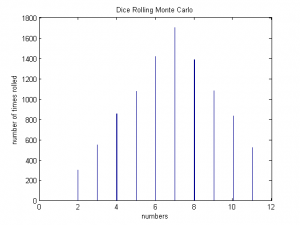
The primary goal of this week was to further our understanding of the Monte Carlo method works. To do this we researched basic modes of how the Monte Carlo method operates. The Monte Carlo method relies on the repeated random sampling to obtain numerical results. We decided to demonstrate how this method can be used to illustrate the distribution of numbers of two dice rolled for an arbitrarily number of times. 

As expected, 7 is rolled the most amount of times.

One of the most basic Monte Carlo methods is the calculation of the value of pi. Look at the following picture, in which a black unit circle is inscribed into a white square: 

We know that the ratio of the area of the circle to that of the square is pi/4. If you need to prove this to yourself, simply divide the area of a circle by that of a square whose sides are twice the length of the circle’s radius. Now, imagine that you dropped a series of evenly and randomly distributed darts across the image. If you counted them, the number of darts within the circle should be about pi/4 times the amount of total darts dropped. It is much easier to simply count these darts than to try any other mathematical measurement. The following code allows us to simulate this scenario by randomly selecting coordinates within the image above. If the randomly selected coordinate has a value of 0, it is black and thus it is counted as having landed in the circle. Most of the trials yield a value of about 3.09, relatively close to pi. We believe that it is off because MatLab is not able to perfectly represent a circle as values in an array.

We then began to research basic option trading techniques. Option trading is a large field in the world of finance and uses computer simulations to traders. To start it was necessary to understand what an option is. The definition from Aswath Damodaran gives a simple, and concise answer: “An option provides the holder with the right to buy or sell a specified quantity of an underlying asset at a fixed price (called a strike price or an exercise price) at or before the expiration date of the option.” To fully understand this definition, it is critical to know that an underlying asset simply means a stock or a portfolio for our purposes.

Option trading typically uses binomial trees or the Black-Scholes method. The Black-Scholes method was published in 1973 and won the Nobel Prize in Economics in 1997, is a way of finding the end price of underlying asset given specified parameters. These parameters include: the strike price, K, the asset price, S, the volatility given by the symbol $\sigma$, the risk free interest rate, r, and the time until maturity T. The Black-Scholes model can be used for two different types of options, a put option and a call option. A call option provides the holder the right to buy the underlying asset at the specified strike price until the maturity date. Conversely, a put option gives the holder the right to sell an underlying asset at the strike price at any point until the maturity date.

For a less technical definition, lets say stock A is being traded for 10 dollars and you can purchase the call option for 2 dollars giving you the right to sell stock A for 10 dollars (the strike price). You believe that stock A will go up to fifteen dollars in a month, so you spend 200 dollars on 100 shares. Fortunately stock A has gone up to 20 dollars, so now you invoke your right to purchase 100 shares at 10 dollars each and then immediately sell stock A. This gives you a profit of 10 dollars a share giving a net profit of 800 dollars because we must take into account the 200 dollars you spent on the call option.  The Black-Scholes model is below:

(1)  

where

(2)  

and

(3)  

$N(d_1)$ is the standard normal distribution of $d_1$ and $N(d_2)$ is the standard normal distribution of $d_2$.

In our code we found the call option for a European option because it is slightly easier to code. For the parameters: $\sigma$ = .3, K=4, S=2, T=3, and r=.4 we get the call option price from the Black-Scholes model is .86415 and from the Monte Carlo method we get .86509. The Monte Carlo method provides a powerful way to check that our solution to the Black-Scholes model is correct. In our case we use an extremely large amount of random numbers. To check our example we encourage you to run our code, which can be downloaded at the link provided at the bottom of the page. Our code runs for the European Call Option and can be checked against: http://www.erieri.com/blackscholes.

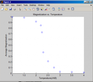
A more advanced Monte Carlo method is used to solve an ising model that represents the spin states of electrons in a magnetic material. Here, we have defined the “isinggrid” to represent a system of interdependent spins. These spins naturally tend to align themselves in the same direction, and thus we have started with a ferromagnetic system in which all spins are aligned. We then simulate stochastic changes in the system that occur because of energy added by the temperature in a heat bath. As temperature rises, the greater there is that one of the spins will orient itself in a way that requires adding energy to the system. This is because the extra heat from the increased temperature supplies extra energy. We have also accounted for the spins at the edges of the grid by applying periodic boundary conditions that allow even spins on the edge to interact with four neighbors instead of two or three. We iterate through 11 temperatures in this example, calculating the overall magnetization for each one. This magnetization, M, is the average magnetization calculated 5000 times by the stochastic Monte Carlo process. If a spin flip results in a decrease in energy of the system, it occurs. If it increases the energy, the program generates a random number and then compares it to a parameter set by the temperature. Below is the average magnetization for each temperature that we tried:

As we can see, there is a very sharp drop off in Magnetization upon reaching a certain temperature, which we will calculate the exact value of by next week. This is a good step in our project, as it is important for us to get used to working with stochastic and semi-stochastic systems. Our financial models will involve similar sorts of ideas.

Link to our code: https://drive.google.com/folderview?id=0B01Mp3IqoCvhflF5azV4bHY2V0c3Vks0VXVyQkIxcnR4RmFaNDhVWEQtZGZSR2t6V2VWOHc&usp=sharing

New References:

1. The Black and Scholes Model: http://bradley.bradley.edu/~arr/bsm/pg04.html

2. Aswath Damodaran http://people.stern.nyu.edu/adamodar/pdfiles/option.pdf

3. Bruce Mizrach  http://snde.rutgers.edu/pubs/[42]-2010_Handbook.pdf