Category Archives: QM

Projects in Introductory Quantum Mechanics

Photobleaching of Methylene Blue

Background:

Photobleaching is the photochemical alteration of a dye or fluorophore molecules that removes its ability to fluoresce. This is a chemical reaction initiated by the absorption of energy in the form of light, with the consequence of the creation of transient excited states with differing chemical and physical properties¹. It most commonly occurs in fluorescence microscopy, where the over excitation of the material or overexposure causes the fluorophore to permanently lose its ability to fluoresce due to the photon-induced chemical damage and covalent modification². However, scientists have newly developed the ‘bleaching-assisted multichannel microscopy’ (BAMM) technique which allows them to manipulate the rate of photobleaching in order to help differentiate fluorophores³. Because the overcrowding of fluorophores attached to different cell targets prove to be a major limitation in imaging, this technique allows researchers to use photobleaching to differentiate between fluorophores rather than the current technique that relies on the different fluorescent emission colors for labelling. The varying rates of photobleaching, or photostability, for the different types of fluorophores allows for this new kind of differentiation. The once weakness of the fluorescent microscopy process is now seen as a strength that allows for increased identification of cellular targets.

Most students are introduced to photobleaching in introductory Biology courses, where the process is exploited to study the diffusion properties of cellular components in molecules by observing the recovery or loss of fluorescence to a photobleached site. The observed changes are due to the change of states from electron excitation via intersystem crossing. Studying the movement of electrons via transitions from the singlet state to the triplet state gives us a better conceptual grasp on the photobleaching process with a molecular focus on energy levels and the wavefunctions of the different spin states. The selection rules describe whether a quantum transition is considered to be forbidden or allowed. This means that not all transitions of electrons are observed between all pairs of energy levels, with “forbidden” being used to describe highly improbable transitions. I will further explore what it means for electrons to change state and which kind of transitions are more probable than others by studying the selection rules and the principles that support their claims. The applicational experiment that I performed, the photobleaching of methylene blue, demonstrates these reactions in real time through color intensity observations.

The Selection Rules

The Laporte Selection Rule

The Laporte selection rule states that the donor orbital and acceptor orbital of the electrons in a transition must have different symmetry or cannot be of the same orbital: (s →s); (p →p); (d →d); (f →f). Additionally, the Laporte allowed transitions allow for (Δ l = ± 1) changes in angular momentum quantum number (1).

(1)

It indicates that transitions with a given set of p or d orbitals are forbidden if a molecule has a center of symmetry or is centrosymmetric. The selection rule determines whether the transition is orbitally allowed or forbidden. If the integral of the transition moment does not contain the totally symmetric representation, the transition is forbidden.

Transitions are only detectable when the transition moment dipole is nonzero and when the wavefunctions include the initial and final states which contain both the electronic and nuclear wave functions (2). The Born-Oppenheimer approximation points out that electronic transitions have a much smaller time scale than nuclear transitions; because of this and the fact that these transitions in question are electronic, the nuclear motion is ignored (3). This approximation is done because we assume that these transitions are instantaneous, so there is no change in the nuclear wavepacket. The Franck-Condon principle is a direct consequence of this approximation, which will be further explored later.

(2)

(3)

Fermi’s Golden Rule (4), which describes the transition rate or probability of transition per unit time from one eigenstate to another and is only allowed if the initial and final states have the same energy, allows M, the electric dipole moment operator to replace the time dependent Hamiltonian (5), giving that final transition moment integral that describes electronic transitions from ground to excited states (6). This integral is equivalent to the probability of a transition taking place. Since the integral must be non-zero for the transition to occur, the two states must overlap, as per the Franck-Cordon principle which states that the probability of electric transition is more likely if the wavefunctions overlap.

(4)

(5)

(6)

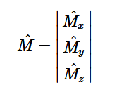
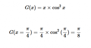
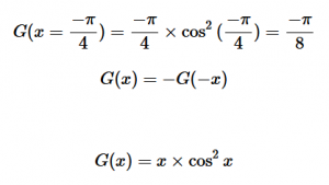
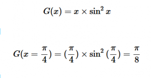
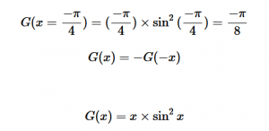
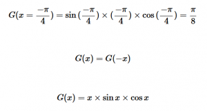
For solving the transition moment integral, the electric dipole moment operator can be rewritten with Cartesian axes (7). Simulating calculations of transitions with M being an odd function between even states (8) , between odd states (9), and even and odd states (10) show that transitions between two similar states are forbidden since the final result is an odd function. Even functions may be allowed transitions but to determine which are totally symmetric, cross products between the initial and final states with the electric dipole moment operator should be worked out.

(7)

Spin Selection Rule

The spin selection rule states that the overall spin S of a complex must not change during an electronic transition (Δ S=0) or (Δ m_S = 0). The spin state or spin of the excited electron coincides with the number of unpaired electrons; the singlet state having zero unpaired electrons and triplet state having two unpaired electrons. The overall spin state must be preserved, so if there were two unpaired electrons before transition, there must be two unpaired electrons in the excited state as well (Figure 1).

Figure 1: The allowed transition shows the transition of states in which the spin remains the same, with one unpaired electron on either side, a doublet to a doublet state. The forbidden transition shows the transition of a triplet state, where there are two unpaired electrons to an excited singlet state where there are no unpaired electrons. The loss of preservation of spin state of the molecule makes the transition forbidden.

The absorption of higher frequency wavelengths, which come in the form of photons or other electromagnetic radiation, excite electrons into higher energy levels. Electrons in general occupy their own states and follow the Pauli Exclusion Principle, which states that no two electrons in an atom can have identical quantum numbers and only two can occupy each orbital but must have opposite spins. The Exclusion Principle acts primarily as a selection rule for non-allowed quantum states. Equation 11 shows the probability amplitude that electron 1 is in state “a” and electron 2 is in state “3”, but fails to account for the fact that electrons are identical and indistinguishable. We know that particles of half-integers must have antisymmetric wavefunctions and particles of integer spin must have symmetric wavefunctions. The minus sign in equation 12 serves as a correction to equation 11. This new equation indicates that if both states are the same, the wavefunction will vanish, since both electrons cannot occupy the same state.

Ψ= Ψ1(a) Ψ2(b) (11)

Ψ= Ψ1(a) Ψ2(b) Ψ ± Ψ1(a) Ψ2(b) (12)

Singlet to Triplet Transition

When an electron in a molecule with a singlet state is excited to a higher energy level, either an excited singlet state or excited triplet state will form. A singlet state is a molecular electronic state where all the electron spins are paired. An excited singlet state spin is still paired with the ground state electron. The pair of electrons in the same energy level have opposite spins as per the Pauli exclusion principle. In the triplet state, the spins are parallel; the excited electron is not paired with the ground state anymore. Excitation to the triplet state is a “forbidden” spin transition and is less probable to form. Rapid relaxation of the electrons allow the electrons to fluoresce and release a photon of light, falling down to the singlet ground state level, which is known as fluorescence.

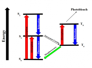
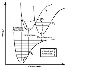
Intersystem crossing occurs when some molecules transition into the lowest triplet state which is at a higher spin state than the excited singlet state but has lower energy and experiences some sort of vibrational relaxation. In the excited triplet state, the molecules could either phosphorescence and relax into the ground singletstate, which is a slow process, or absorb a second phonon of energy and excite further into a higher energy triplet state. These are the forbidden energy state transitions. From there it will either relax back into the excited triplet state or react and permanently photo bleach. The relaxation or radiative decay of the excited triplet metastable state back down to the singlet state is phosphorescence where a transition in spin multiplicity occurs (Figure 2).

Figure 2: Energy diagram showing the transitions the electrons undergo when gaining and releasing energy. Although the first excited singlet state, S1, has a lower overall Spin State (S=0), the intersystem crossing shows that the triplet state has lower energy (S=1). The photobleaching pathway via the triplet state is highlighted as further excitations in triplet states are more likely to bleach fluorophores.

To further clarify, intersystem crossing (ISC) occurs when the spin multiplicity transforms from a singlet state to a triplet state or vice versa in reverse intersystem crossing (RISC) where the spin of an excited electron is reversed. The probability is more favorable when the vibrational levels of the two excited states overlap, since little or no energy needs to be gained or lost in the transition. This is explained by the Franck-Condon principle. States of close energy levels and similar exciton characteristics with same transition configurations are prone to facilitating exciton transformation⁴.

Zeeman Effect

Transitions are not observed between all pairs of energy levels. This can be seen in the Zeeman effect, a spectral effect, of which the number of split components is consistent with the selection rules that allow for a change of 1 for the angular momentum quantum number (Δ l = ± 1) and a change of zero or of one unit for the magnetic quantum number (Δ m_l = 0, ± 1). The orbital motion and spin of atomic electrons induce a magnetic dipole, where the total energy of the atom is dependent on the orientation of this dipole in a magnetic field and the potential energy and orientation is quantized. The spectral lines that correspond to transitions between states of different total energy associated with these atoms are split because of the presence of a magnetic field⁵. This was looked for by Faraday, predicted by Lorentz, and observed by Zeeman.

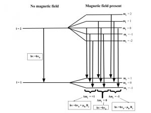
The Zeeman effect or “normal” Zeeman effect results from transitions between singlet states while the “anomalous” Zeeman effect occurs when the total spin of either the initial or final states is nonzero with the only tangible difference between the two being the large value of the electron’s magnetic moment of the anomalous effect. (Figure 3). For singlet states in the normal Zeeman effect, the spin is zero and the total angular momentum J is equal to the orbital angular momentum L. The anomalous Zeeman Effect is complicated by the fact that the magnetic moment due to spin is 1 rather than 1/2, causing the total magnetic moment (14) to not be parallel to the total angular momentum (13).

Figure 3: The normal Zeeman Effect occurs when there is an even number of electrons, producing a S = 0 singlet state. While the magnetic field B splits the degeneracy of the m_l states evenly, only values of 0 and ± have transitions. Because of the uniform splitting of the levels, there are only three different transition energies.

(13)

(14)

Franck-Condon Principle

The Franck-Condon principle is a rule used to explain the relative intensities of vibronic transitions, in which there are simultaneous changes in vibrational and electronic energy states of a molecule due to the absorption of emission of photons. This principle relies on the idea that the electronic transition probability is greater if the two wave functions have a greater overlapping area. The principle serves to relate the probability of a vibrational transition, which is weighed by the Franck-Condon overlap integral (15), to the overlap of the vibrational wavefunctions.

(15)

Figure 4: Energy state transitions represented in the Franck-Condon principle energy diagram. The coordinate shift between the ground and excited states indicate a new equilibrium position for the interaction potential. The shorter arrow indicating fluorescence into the ground state indicates that a longer wavelength and less energy than what was absorbed into the excited state.

Classically, the Condon approximation where there is an assumption that the electronic transition occurs on a short time scale compared to nuclear motion allows the transition probability to be calculated at a fixed nuclear position. Since the nuclei are “fixed”, the transitions are considered vertical transitions on the electronic potential energy curves. The resulting state is called a Franck-Condon state.

The nuclear overlap between state transitions can be calculated by using the Gaussian form of the harmonic oscillator wavefunctions.

Overlap of Zero-zero transition S₀₀

Using the harmonic oscillator normalized wavefunctions for the ground (16) and excited electronic states (17) where α = 2πmω/h, Re is the equilibrium bond length in the ground state and Qe is the equivalent for the excited state, the nuclear overlap integral can be determined (18). Expanding the integral and completing the square gives us equation (19). Simplifying the Gaussian integral gives us the overlap of the zero-zero transition states (20).

(16)

(17)

(18)

(19)

(20)

Overlap of S₀₁Transition

Solving for the zeroth level of vibration in the ground and the first excited vibrational level of the excited state, S₀₁is similar to how S₀₀was solved, using the equation (21) again. Using (16) and (22) as the zeroth and first excited state wavefunctions for the ground and excited states, the overlap can be found (23). Simplifying similarly to the previous walk-through, equation 24 shows the simplified overlap of the vibrational levels value.

(21)

(22)

(23)

(24)

Applicational Experiment: Photobleaching of Methylene Blue

Experimental Background:

A HeNe laser emits a wavelength along the visible spectrum that is absorbed by the methylene blue causing a reaction known as photobleaching. The methylene solution will take on a colorless appearance due to the absorption of the photons, exciting the electrons into new spin state. A singlet spin state, which quantifies the spin angular momentum in the electron orbitals, will either transition into a ground state or into an excited triplet state, both of which have lower energies. The transition into the triplet state involves a change in electronic state which increase the states lifetime, allowing it to be a strong electron acceptor.

The colorless appearance of the irradiated solution is due to the oxidation of the triethylamine due to the excited triplet state. The ‘photobleaching’ of the methylene blue, as more easily seen from placing and removing the solution from sunlight, is not permanent and functions more as a decay in which the electrons jump to high energy excited states and fall back down to its ground state. Using a laser has a longer lasting effect on the solution, as more waves of higher frequency are absorbed, slowing down the time it takes for the solution to return to its original state.

Experimental Procedure and Results:

With supplies provided by the Chemistry department and Professor Tanski, I was able to create the methylene, triethylamine mixture. Triethylamine is a chemical that has a strong odor so working under a hood is essential. (Or else the whole building would have to evacuate cause of the smell if it fell!) While wearing googles in a chemical hood, I measured out 10mL of water with a graduated cylinder into a 10mL vial, added 1-2mg of methylene blue powder, which is such a small amount that it was very difficult to weigh out, and added 5 drops of triethylamine. I pipetted approximately 0.75mL of the sample into three 1mL vials, labelled for photobleaching by the red HeNe laser, green HeNe, or as the experimental control. The remaining liquid was meant to examine the effects of natural sunlight on the methylene solution. The dark blue solution was meant to lighten in color due to the suns less intensive photobleaching properties. Placing the solution back in darkness would allow for the excited electrons to fall back down to the ground state and return to its original color, since the energy absorbed wasn’t high enough to cause permanent photobleaching. For some reason, my solution did not have a reaction to the sun as expected, which was probably due to me not mixing the solution well enough before I distributed it into three other vials. In comparison to my predictions with the reactions using the HeNe lasers, the sunlight would take longer to turn colorless but would take a very short amount of time to return to its original color, since the excited electrons are not falling from a high energy level.

I then visited the Michelson Interferometer and Fourier Transform experimental set up that had the red and green HeNe lasers that I required. I darkened the room to lessen the effects of stray light, but since the shades don’t completely block out the sunlight, I couldn’t reach full darkness. With one laser on at a time, I placed the vial directly in front of the beam, hoping to irradiate the appropriate vial with the laser until the color changed. Unfortunate, my vials did not change color at all, even after holding them to the beam for thirty minutes straight. As I mentioned earlier, this error was probably due to my lack of proper mixing of the solution. What was meant to happen was that the energy received from each laser was supposed to turn the solution clear in color. I would have predicted that the red laser, due to higher frequency and higher energy in the photons, would have caused the solution to become colorless quicker and after keeping the vials in darkness, would take longer to return to its original dark blue color since the excited electrons have higher energy levels to fall from.

Overview:

Reproducing the photobleaching of methylene blue allowed me to apply my knowledge about the electron spin states, specifically singlet and triplet states, and the observable transitions that was suppose to take place in my experiment. I had learned a bit about spin states in Organic Chemistry but studying them from a Physics standpoint is very different, requiring further conceptual questioning about why certain transitions were more likely than others. My in-depth look into the rules and principles behind the seemingly simple excitation of electrons into different states was very interesting and a great experience, prying apart every argument, looking for the basis of which each statement came from, and learning the conceptual theory as well as the mathematics that back it up. Thank you Professor Magnes for a great semester!

(1) https://www.britannica.com/science/photochemical-reaction

(2) https://www.microscopyu.com/references/fluorophore-photobleaching

(3) https://phys.org/news/2018-06-fluorescence-microscopy-bamm-treatment.html

(4) https://www.ncbi.nlm.nih.gov/pmc/articles/PMC5524908/

(5)http://bcs.whfreeman.com/webpub/Ektron/Tipler%20Modern%20Physics%206e/More%20Sections/More_Chapter_7_2-The_Zeeman_Effect.pdf

Modeling the Potential Barrier in the Esaki Diode

Introduction

The Esaki tunnel diode is a semiconductor p-n junction that uses the phenomenon of quantum tunneling to its advantage. The junction between the two doped semiconductor materials creates a potential barrier between the valence band of the p-type material and the conduction band of the n-type material. If the potential barrier is thin enough, and depending on the bias of the junction, individual electrons can tunnel either “forward” or “backward” through the potential barrier, collectively creating a current. In fact, the tunnel diode exhibits the unique characteristic of having negative resistance at particular levels of forward bias. I have approximated this potential barrier in order to perform the sort of one-dimensional analysis we did in class. My goal is not to find accurate numerical quantities that describe a real-life Esaki diode, but rather to apply what we learned about potential barriers in class in order to demonstrate the relationship between the dimensions of a barrier and the transmission coefficient of an incident wavefunction in the context of a real device.

Background

Whereas electrons in individual atoms have discrete, quantized energy levels, electron in solids interact with each other in such a way as to form continuous “bands” of allowed energy. In semiconductors, we focus on the valence and conduction bands. At absolute zero, the states in the valence band are full, but optical or thermal excitation can excite electrons up to the conduction band – a necessary condition for the semiconductor to conduct electricity. When an electron is excited in this way, it leaves behind a corresponding “hole” – simply the absence of an electron – which can be thought of as having the electron mass with opposite charge. Together these are known as an electron-hole pair (EHP).

Semiconductors are often doped, meaning an otherwise pure semiconductor material has been injected with a small concentration of atoms that allow either for more electrons (n-type), or more holes (p-type). Every semiconductor has a fermi energy, below which almost all states are occupied, and above which nearly all states are vacant. An undoped semiconductor has fermi energy approximately halfway in between the valence and conduction bands, but n-type doping raises the fermi energy and p-type doping lowers it. The Esaki diode uses degenerate materials, which are doped so heavily that the fermi energy is outside the band gap.

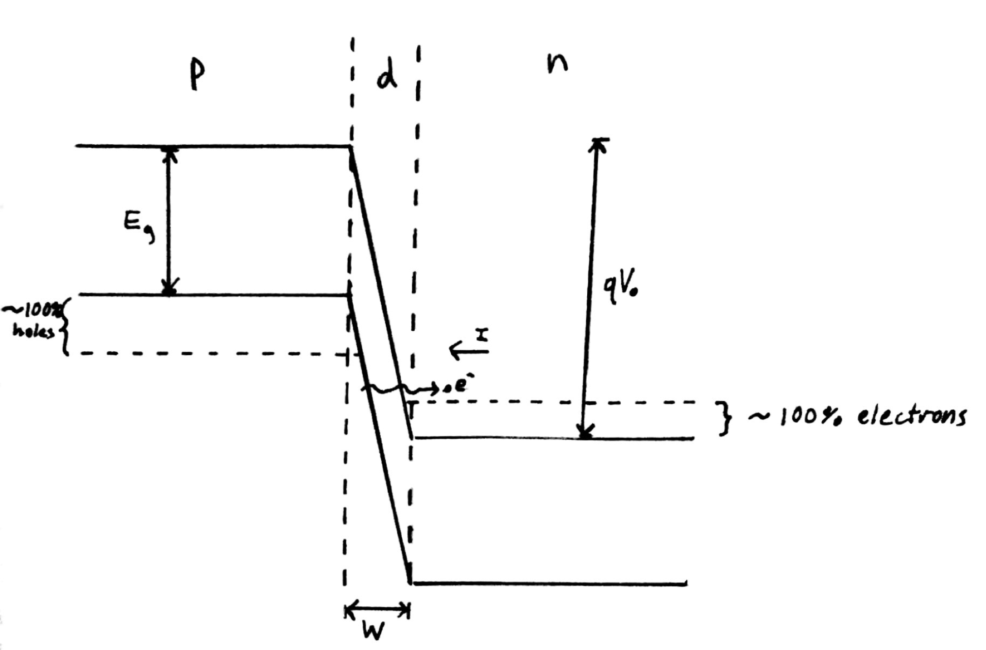
When p- and n-type semiconductors are joined together, they form a junction. At equilibrium, the fermi energy must remain constant, which causes the bands of each material to bend with respect to one another by a quantity qV₀, called the contact potential (times the elementary charge), over a depletion region of width W. When a bias, or voltage, is applied to the junction, the fermi energy can then have different values //on either side.

The tunnel diode is simply a p-n junction with the correct conditions for tunneling to occur. First, the contact potential is high enough that the valence band of the p-type region overlaps the conduction band of the n-type, so that an electron can tunnel through the potential barrier from one side to the either. This condition becomes hard to maintain at certain levels of forward bias – as the voltage increases and the respective valence and conduction bands move out of alignment, the tunneling becomes less likely per electron, resulting in a weaker current. Second, the materials must be degenerate to create regions of empty states. Third, the junction must have a forward or reverse bias, so that the fermi energies are unequal and thus an empty state can exist across from a filled state. Fourth, the width of the potential barrier must be narrow enough for electrons to be able to successfully tunnel from one side to the other. It is this last condition that we will be modelling.

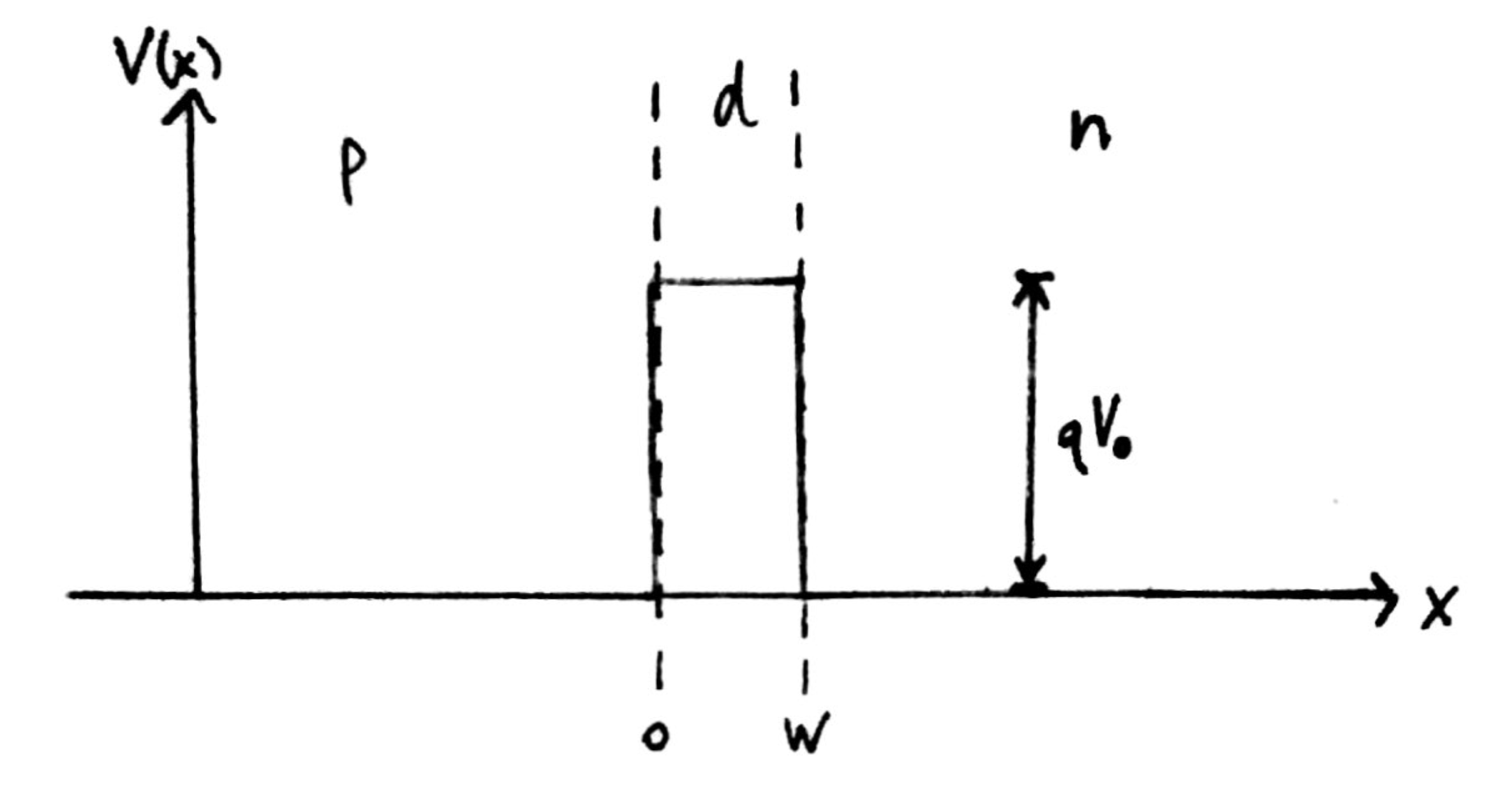
Fig. 1: Band diagram representing Esaki diode under tunneling condition. The diode is reverse biased, allowing an electron on the p side to tunnel across to an empty state on the n side.

1-Dimensional Quantum Model

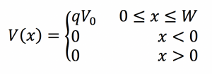
The Esaki diode’s potential barrier looks different from the barriers we’ve examined in class, in that it actually comprises two energy functions. Counterintuitive as this is, the important aspects of the barrier are its width, approximately W, and its finite height, qV₀. Thus, since the “sides” of the barrier are nearly vertical when highly doped, we’ll approximate it as a simple rectangular barrier with the same dimensions. The potential on either side can simply be 0.

Fig. 2: Rectangular potential barrier representing Esaki diode barrier. This model has the same height and width as the real barrier.

An electron in this system has a wavefunction that satisfies the time-independent Schrödinger equation:

where

For the p and n regions, we can use the standard free particle solutions, assuming the electron is incident from the left:

with

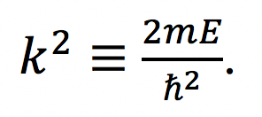
The depletion region’s TISE can be written as

So the solution is given by

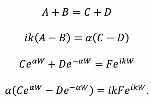
In order to determine the arbitrary coefficients, we must impose the boundary conditions, which state that the wavefunctions and their first derivatives must have continuity over each boundary. We get the following system of equations:

With some tedious algebra, we can solve for A in terms of F:

Now we can calculate the transmission coefficient:

Simplify and plug in original values for α and k to get expression in terms of given quantities:

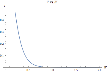
This expression makes sense, because the limit as W goes to infinity is 0, and the limit as W goes to 0 is 1, meaning the electron is only likely to tunnel for small W. Note also that as the contact potential V₀ goes to infinity, T goes to 0, as we would expect from an infinite potential well. Initially, we assumed the electron was incident from the p-side, as in the reverse bias case, but the mirror symmetry of our model means that as far as the barrier is concerned, we can expect identical behavior for an electron incident from the n-side.

Fig. 3: This graph was produced in Mathematica using rough estimates for the energy values in the T equation. The numbers on the axes are not intended to represent actual quantities, and the graph merely suggests the shape of the function.

Conclusion

Although this model is very much an oversimplification of what the potential barrier in an Esaki diode actually looks like, it demonstrates the sort of behavior we would expect from the real thing, namely the behavior of the transmission coefficient with respect to the extremes of barrier width. Although the key characteristics of the tunnel diode are dependent on the doping of the two semiconductor materials, which falls outside the scope of this course, the rectangular barrier model focuses purely on the quantum mechanical process that lies at the core of this diode’s function.

Sources

Goswami, Amit. (1997). Quantum Mechanics. (2nd ed.). Waveland Press, Inc.

Griffiths, David J. (2004). Introduction to Quantum Mechanics (2nd ed.). Prentice Hall.

Streetman, Ben G., Banerjee, Sanjay Kumar. (1988). Solid State Electronic Devices (7th ed.). Pearson.

QUANTUM SHOT NOISE

INTRODUCTION
For my project, I worked on the shot noise experiment and explained the concept of shot noise from a quantum mechanical perspective. The experimental component was necessary to understand how shot noise can be observed and measured. It was also necessary to model how transmission probabilities change with a changing voltage. The quantum mechanical component was necessary to describe an application of tunneling through step potential and its effects.

OVERVIEW OF SHOT NOISE
Noise can be observed when an electric current is generated from random independently generated electrons. Shot noise exists in certain macroscopic electric currents and can only be observed when the electric current is amplified thereby amplifying the noise. Shot noise is a result of the discreteness of electrons where the number of electrons arriving over a given period can be described using the Poisson distribution [3]. The randomly generated electrons create an uncertainty in the arrival of electrons. The standard deviation in the number of electrons arriving during that period is given by the square root of the number of electrons arriving for that period [3]. The statistical fluctuations in the arrival of electrons result in statistical fluctuations in the charge about its mean. These fluctuations are what we refer to as noise and can be observed through the shot noise experiment [3].

Fluctuating currents have also been theorized by Landauer [1] to result from random transmission of electrons from one terminal to another as individual electrons move across a potential barrier. The conductor can be modelled as N independent channels arranged in parallel to create the conducting wire [2]. In this case, each scatter-site can be thought of as a gap in the conductor. Electrons tunnelling through each independent channel, have a transmission probability Tn [2]. The transmission probabilities can be computed using the scattering matrix approach or by using Landauer’s formula.

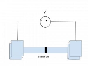
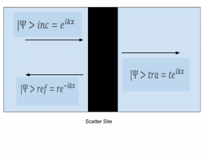
This can be modelled as shown in Figure 1 below where electrons tunnel through the scatter site when moving from one terminal to the other. The wave packet tunnelling through the scattering site from the left of the scatter site to the right of the scatter site generates a current pulse. Electrons can tunnel from the right of the scatter site to the left of the scatter site, or vice-versa. The tunnelling of electrons is random resulting in fluctuating currents which we observe as noise [2].

Figure1: a) Conducting wire modelled as a channel between two terminals with scattering sites through the channel b) Scatter site showing incident, reflected and transmitted wave functions for an electron approaching the scatter site from the left

METHODS
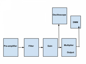
The shot noise experiment is set up as shown in the block diagram below. A photocurrent ejects statistically independent photoelectrons. The current is passed through a load resistor producing a dc voltage. In the low-level electronics (LLE), there is a high pass filter that passes frequencies above the cutoff frequency. The current is passed through an op-amp with a gain (G=100) in the preamplifier. The output of the pre-amplifier is then sent to the high-level electronics that includes a low pass filter and a gain (G=6000). The output from the HLE is an average amplified noise voltage. The frequency bandwidth that the high pass and low pass filter create determines the period over which statistically independent arrivals of electrons can be made. This amplified noise voltage can be calculated, and theoretical results compared to the experimental results.

Figure 2: Block diagram for the shot noise experiment

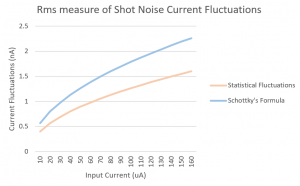
For this project, only the theoretical results were considered. An expression for the standard deviation in the current was used to calculate the rms measure of current fluctuations. These fluctuations were also calculated using Schottky’s formula (Eq 1). The two methods were used to compute the expected current fluctuation rms measurements [3].

The model used to compute the expected current fluctuations was used to compute the sum of transmission probabilities of the N independent channels in the conductor. Landauer theorized that the time-averaged current can be computed from the conductance multiplied by the voltage and the sum of the transmission probabilities as shown in equation 3 below [1]. The sum of transmission probabilities was therefore calculated from the time-averaged current and the voltage using Eq 2.

RESULTS
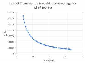
Figure 3 below shows the results of the rms measure of the current fluctuations calculated using both Schottky’s formula and from the standard deviation in the current. From the graph below, the Schottky formula can be approximated as a suitable measure of shot noise current fluctuations as the current fluctuations are nearly equal. The average power transmitted by a noise source is proportional to the shot noise amplitude and is therefore proportional to the average dc current and to the as seen from Eq 1 and Figure 3 below. The average power is also proportional to the bandwidth frequency. Figure 4 below shows how the sum of transmission probabilities of n channels changes with changing voltage.

Figure 3: Rms measure of current fluctuations Figure 4: Transmission probabilities vs Voltage

DISCUSSION
The sum of transmission probabilities decreases exponentially with an increased voltage as seen in Figure 4 above. This corresponds to what we expect from Ohms Law and Landauer formula where conductance (1/R) increases with increased transmission probability, and conductance is inversely proportional to voltage. It, therefore, follows that transmission probability decreases with increased voltage. Another approach to computing transmission probabilities is through the use of the scattering matrix.

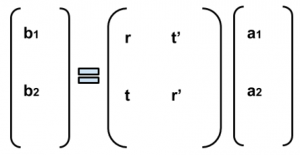
The scattering matrix has extensively been used to describe quantum transport by describing the relationship between electrons approaching a scatter site from the left and electrons approaching a scatter site from the right [2]. The wave equations for electrons approaching the scatter site from the right are similar to those shown in Figure 3 however the reflection and transmission coefficients r’ and t’ respectively [2]. The scattering matrix shown below is thereby necessary to calculate amplitudes of the waves approaching the scatter site from the left and those approaching the scatter site from the right. This offers an alternative way to compute transmission and reflection probabilities.

CONCLUSION
In conclusion, this study has found that fluctuations in an electric current can be attributed to the discreteness of electrons where we can use Schottky’s formula to calculate current fluctuations. It was also found that noise can be attributed to the uncertainty introduced by electrons tunnelling through a scattering site. The probabilities of transmission can be calculated using Landauer formula or could be found using the scattering matrix approach. The Schottky formula was found to closely match the count statistics approach to compute current fluctuations. It was also found that the sum of transmission probabilities decreased with increasing voltage.

REFERENCES
[1] Datta, S. (1995). Electronic transport in mesoscopic systems. Cambridge: Cambridge University Press.
[2] Lesovik, G. B., & Sadovskyy, I. A. (2011). Scattering matrix approach to the description of quantum electron transport. Physics-Uspekhi,54(10), 1007-1059. doi:10.3367/ufne.0181.201110b.1041
[3] Shot Noise Experimental Manual. NF Rev 1.0 9/1/2011. Vassar College

Quantum Companion: Introduction of topics through accessible programming-d

Motivations

The material that is covered and encompassed in an introductory quantum mechanics course can prove to be daunting and impressive to new comers. This is alleviated by endless class discussions and hours digging through stack exchange after stack exchange looking for further explanations. A central resource for related course material could serve as both a time saver and an interest promoter.

Overview

Through some programming, the hope was to create a standalone mobile application for use in accessing this cache of materials. Utilizing online HTML seemed to be the most straightforward approach in incorporation of this material for multiple platforms. Materializing all of the resources necessary to go through a course in quantum mechanics is a very relative goal, so creating space for at least the main concepts served as the most attainable goal. I was able to partially succeed in doing this, though not to the full extent than had predicted during the introductory stages.

A selection of these course topics was made after some discussion among fellow members of this introductory course. Spacing out topics covered and going over a few that were not discussed in depth served as a more than daunting task. The shear amount of information present lead to a thinning of topics, and an emphasis on the ones more visually appealing to discuss.

In the development of this course companion, I consulted several members of the Vassar CS department to coordinate the application of several action-related components of my proposed code. After several de-bugging sessions, I was able to integrate this into an independent URL and I later stored databases through WordPress.

I had also intended to provide some real-time walk though examples of some selected topics, but the production aspects of these films proved very low after I attempted to use equipment loaned out through media resources.

Navigation walk through

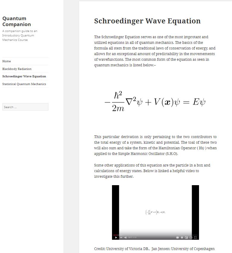
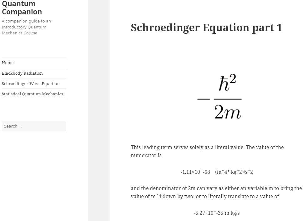
These screenshots serve as representations of a single line of inquiry for the project. A multitude of others are programmed in, but are not represented here.

The first beginning page of the collection starts with a brief introductory statement of purpose and is framed by a list of available resources discussing several of the topics.

Homepage sweet home

Each of these pages offer a brief representation and provide more links to further expand into detail depending on the total variables present in the equation.

First Reference Page

First Equation example. These pages are represented for components of equations.

End Results

The culmination of this project resulted in less than my initial projections . Keeping with the entirety of a course subject on a single page is, as I’m sure any instructor knows, quite the task. Even with weeks of time leading up to the execution, creating realistic goal timelines, and collaborating with more experienced programmers; this was a tall order to fill. The finished product of all of these hours of effort and error resides at QuantumCompanion.xyz . I hope stands as a strong representation of the time and commitment to this cause.

If I were to recreate this quantum site again, I would spend less of my time focusing on the programming side of the project. A significant portion of my time was squandered pouring over code instead of building better content. In the future, I would like to expand on this idea of a cumulative website and include more original content. Having video presentations, I feel would also add to the overall effectiveness of the site, and, given another attempt at using recording equipment, I would hope to deliver on this aspect of the project.

Quantum Key Distribution: Methods, Mechanics, and Development

Introduction
Just as in other areas in the field of computer science, making the leap from classical- to quantum-mechanical properties as a basis for software developments introduces an entirely new level of possibility for real-world applications. For example, the basic implications of the concept of the qubit alone are enormous: the possibility of ultra-fast communications, up to the speed of light, as well as the potential availability of coding based on higher-order numeric systems (quaternary, rather than binary information, for example).

The introduction of quantum-mechanical principles to the area of cryptography, likewise, creates the opportunity for immensely powerful encryption protocols. By using basic tenets of subatomic physics, such as the Uncertainty Principle and Bell’s Theorem, computational cryptographers now have the power to create what amount to essentially unbreakable codes. Previously, when classical encryption methods relied on the increasing complexity of mathematical functions, there always existed the threat of an enemy with a more powerful computer able to intercept decipher an encrypted transmission. However, no computer, no matter how strong, is able to simultaneously measure orthogonal quantum eigenstates or preempt the prediction of spin states between quantum-entangled particles. The universality of physical law, in effect, becomes a computational tool in quantum cryptography.

In this project, we will investigate one of the most useful and fundamental processes of quantum cryptography: quantum key distribution (QKD), whereby two communicating parties establish a secret key through quantum-mechanical procedures. We will first examine, after a discussion on the underlying physical and mathematical concepts, the Bennett-Brassard Protocol, published in 1984, which uses polarized photons as transmitted qubits. Following this, we will discuss the other major protocol for quantum key distribution, the Eckert Protocol, published in 1991, which instead revolves around measuring the spin of entangled particles. The project will conclude with a brief discussion of the current development of QKD, including recent experiments and new directions for research.

Key Terms
quantum channel – a path through which quantum information can be transported; in quantum computing this is most often a fiber optic cable that transports photons
classical channel – any form of communication between two parties that does not rely on quantum-mechanical principles

qubit – a unit of information (a binary bit, 0 or 1) which has been encoded in the quantum property of a particle, such as the spin of an electron or the polarization of a photon

Alice – a term for the sending party across a communication channel

Bob – the receiving party of an information transaction

key – a series of bits that is shared between Alice and Bob in order to establish the security of their communication channel; if the two parties can successfully match their secret key, then they know that their communications are secure

Eve – short for “eavesdropper,” a third-party hacker who attempts to intercept communications between Alice and Bob or otherwise compromise the security of their communications channel

one-time pad – an encryption method that combines every data point of a communicated message with a corresponding bit in a pre-established secret key; a key used for a one-time pad should be exactly as long as the message, and discarded and regenerated after every use. The name “one-time pad” refers to Cold War-era espionage, when spies would lay a pad of paper with a written cipher over a message to encrypt it, then destroying the pad.

I. Quantum-mechanical Systems and Photon Polarization

click to open

II. The Bennett-Brassard Protocol

click to open

III. The Einstein-Podolsky-Rosen Paradox and Bell’s Theorem

IV. The Eckert Protocol

V. Experimental Applications of Quantum Key Distribution

References

Bennett, C., F. Bessette, G. Brassard, L. Salvail and J. Smolin, “Experimental Quantum Cryptography,” Journal of Cryptography, Vol. 4, no. 3, 1992, pp. 3-28.

Bennett, C.H. And G. Brassard, “Quantum cryptography: Public key distribution and coin tossing,” Proceedings of IEEE International Conference on Computers, Systems, and Signal Processing, Bangalore, India, December 1984, pp. 175-179.

Eckert, A, “Quantum cryptography based on Bell’s theorem,” Physical Review Letters, Vol. 67, no. 6, 5 August 1991, pp. 661-663.

Goswami, A., Quantum Mechanics, Second Edition, 2003, Waveland Pr Inc.

Griffiths, D.J., Introduction to Quantum Mechanics, 1995, Prentice Hall, Inc.

A Tale of Two Photons: Quantum Entanglement in Vassar’s Physics Labs

By Jay Chittidi (’19), Lab Partner: Ellis Thompson (’20)

“Spooky Action at a Distance” is among one of the phrases that comes to mind for even someone without any experience with quantum mechanics thinks about some of the “paradoxes” of our quantum reality. It’s a phrase coined by Einstein when lecturing about quantum entanglement, and it was a phrase that came to my mind throughout our quantum mechanics class and the project I worked on with Ellis Thompson. We are fortunate to have a lab setup here at Vassar that allows students like ourselves to experiment with quantum entanglement and take real data that can (hopefully) reproduce the quantum mechanical conclusion that Bell’s Inequality does not hold (more on this later).

Warming Up to Entanglement

The critical idea behind entanglement relates to superposition. In class, we have worked a little bit with the idea that particles can exist as a superposition of states, thus involving multiple wavefunctions. For entanglement, two photons can exist in a superposition of the same state, such that a measurement of a property of one is dependent on the other (their wavefunctions collapse to the same state at the same time when observing one of them). In our case, the observable is the polarization state; the down-converted photons are in a superposition of vertical and horizontal polarization. Here’s the punchline — correlated photons will collapse to identical polarizations that we can detect. We call the detected correlated photons our “coincidences.”

The biggest takeaway should be this — the two photons aren’t “communicating” in any way. As one can imagine, if we have two entangled photons on opposite ends of the universe, a measurement of one will determine the state of the other. If the measured photon somehow sent information to it’s entangled partner, that information would have to travel faster than the speed of light in order for instantaneous collapse to occur! Instead, the nature of quantum mechanics is such that they two photons are said to interact “non-locally,” meaning that “communication” isn’t what’s happening here, but a purely quantum phenomena that both doesn’t fit our human understanding of interaction and (thankfully) doesn’t violate relativity.

So what about Bell’s Inequality? To explain that, we need to first consider the consequences of quantum entanglement. If we consider entangled photons at a very large distance apart, we might wonder how it’s possible for the entangled photons to I’ll go over the mathematics description of this briefly (it’s a complicated derivation and outside of the scope of our class). The Clauser, Horne, Shimony, and Hotle (CHSH) version of Bell’s Inequality² applies directly to our own work in that we can substitute for polarization angles and determine whether our own data support or violate the theory of hidden variables to explain quantum entanglement. We can describe our data as follows with the “arbitrarily” defined variable for correlated photons under hidden variable theory:

Here, E is a mathematical description of correlated photons and N is the number of coincidences as a function of the two polarization angles over a given time step. θ1 and θ2 represent the initial polarization angle for each detector, and θ_1⊥ and θ_2⊥ are θ₁ + 90° and θ₂ + 90°. As is evident, we expect that the number of coincidences to be a function of polarization! Then, we consider CHSH Inequality in the following form:

The variable S is a function of E, which we obtain directly from our data. θ₁‘ and θ₂‘ are θ₁+45° and θ₂+45°. The final piece of our work is to say for all hidden variable theories, S ≤ 2. From our data, we hoped to demonstrate that S > 2 and thus that Bell’s Inequality doesn’t hold. The derivation of these equations and extremely complicated and nontrivial, and really just mathematical motions for understanding hidden variables, and thus is outside of the scope of our work.

Our Experimental Setup and More Background

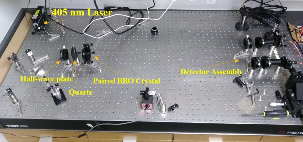
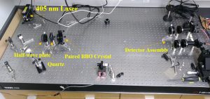
I find that learning about entanglement in the context of our experiment specifically is most insightful. First, we use a violet laser (405 nm) that is intercepted by a half-wave plate that we set to 22.5° (leading to a 45° polarization). Then, we use a quartz plate to phase correct the light before it encounters the paired BBO crystal. Now here is where the “magic” happens. The non-linearity of the paired crystal results in some photons experience (random, probabilistic) phenomenon known as spontaneous parametric down-conversion (SPDC, like ACDC!), wherein one photon emerges from the process as two photons with twice the wavelength (infrared!).

Now, these down-converted photons obey conservation of momentum, and so they both form the same angle with the original beam path. The critical consequence of the conservation of angular momentum is that the polarization of the two photons are orthogonal to the “parent” photon. Further, the emerging photons have a polarization state (either horizontal or vertical) determined by the crystal pair, but we cannot know which crystal specifically results in the polarization state. This results in the two photons existing in a superposition of polarizations until at least one of them is measured. But, the consequences of the SPDC process mean that the same wavefunction describes both photons and thus a measurement of one causes the other photon to collapse into the same state. Hence, this sense of superposition is more than our traditional sense, as the two photons are entangled and correlated.

Equation 3, from Dehlinger and Mitchell¹, represents the state of photons before they are down-converted. θ_l represents the angle from the half-wave plate and Φ_l is the phase shift from the quartz plate. The p subscript denotes that the polarization is from the pump beam.

Equation 4, also from Dehlinger and Mitchell¹, is the state after down-conversion. The subscripts s and i represent the signal (detected) photon and the idler photon. I show these equations simply to demonstrate how after down-conversion, we cannot describe the state of either the signal or idler without considering the other. I point the reader to Ellis’s blog post for more about polarization states in the context of our quantum class, as she uses the Hermitian operator for a quick analysis of the formalism involved.

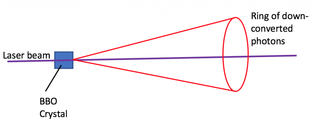
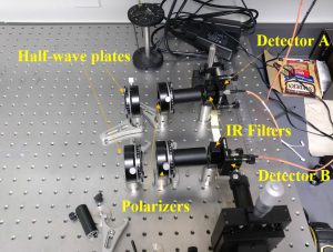
The down-converted photons actually emerge as a cone of infrared light we can detect (see Figure 3), but this also means that the coincident photons are all 180° from each other on the cone! This proved troublesome in our efforts and I’ll mention more later. Before the final leg of their journey, the (hopefully) entangled photons encounter a second half-wave plate, and then a polarizer that is the dependent variable in our experiment. Finally, the photons pass through an infrared filter we use to shield from ambient lighting, and then they reach our photo diode (the detector).

Figure 1: A bird’s eye view of the stage. See above for a detailed description

Figure 2: The detector assembly. Detector B is on an XYZ Transform to aid in alignment. See below for more details.

Figure 3: A diagram in a semi-2D plane of the ring of down-converted photons. Note that the purple beam is exactly in the center of the cone.

Our Struggles

At the beginning of our work, Detector B was quite misaligned. The cone of down-converted photons form a very thin stream, so exploring the parameter space with the detector was a very lengthy and tiresome process. Fortunately, we had the assistance of an XYZ Transform and Professors Daly and Magnes. In December, with a stroke of luck we managed to bring the detector close to alignment by adjusting the angle of the detector while exploring along the y and z axes.

Next, we made many fine adjustments to maximize the number of counts reaching Detector B. We were very systematic with this step, as we were able to realize where on the “circle” of photons we were by observing how the counts reaching the detector changed along the z and y axes. As is evident, laser alignment took the longest time for us!

Our next step was to maximize coincidences, which are not necessarily directly increased by placing our detectors where the down-converted photons are. We realigned the polarizer and half-wave plate in front of Detector B and locked them down, and this improved our number of coincidences significantly. The quartz plate, as mentioned earlier, adjusts the phase of the beam before down-conversion, and so at the suggestion of Professor Daly, we slightly rotated the plate until we maximized coincidences. With this final adjustment, we were finally ready to take data during study break!

Data

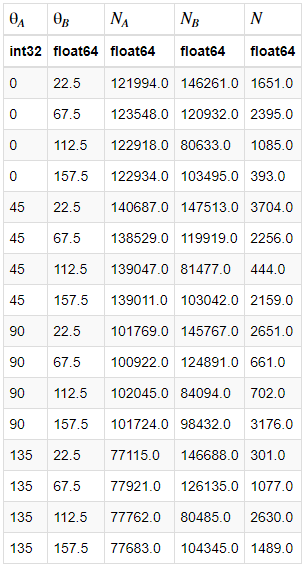
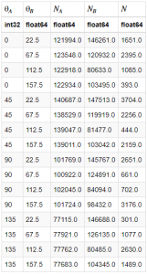
Looking closely at equations 1 and 2 will show that in order to calculate S, we need to measure the coincidences at 16 combinations of polarizations. We will refer to θ₁ and θ₂ as θ_A and θ_B and α and β as these are the formalisms adopted in Dehlinger et al. 2002¹. We choose to do this systematically where we fixed θ_A and went through the angles of θ_B, and rinsed and repeated. Our integration time was 10 seconds, a value that was twice that of which previous students used, but not inappropriate for our work, as saturation and other effects were not present, so we could increase our signal-to-noise. We plot the data in Table 1.

Table 1: A data table resulting from processing our work using Python (and the package Astropy). θ_A and θ_B are the polarizer angles for Detectors A and B, respectively. N_A and N_B are the total counts in each detector over the 10 second period, and N is the number of the counts that were coincidences.

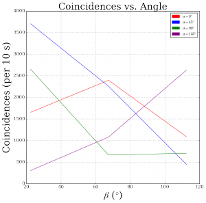
We expect that for any fixed value of θ_A or θ_B, the resulting four measurements of coincidences should be describable by a sinusoid due to the relationship of orthogonality of the states (we expect minima and maxima). Unfortunately, our data do not reflect this as Figure 4 will show.

Figure 4: We plot the number of coincidences as a function of the polarizer angle for Detector B, while holding constant α (we choose to reflect the four values of α with colors). As is apparent, only for α = 0° does our data appear sinusoidal. What we expected were two minima and two maxima for each set of four measurements.

Results

The clear absence of sinusoidal behavior in Figure 4 is a sign that something isn’t quite right. To make this clear, however, we calculate S as described in equations 1 and 2. We report that from our data, we find S = -0.047 ± 0.028, which falls within the prediction of Bell’s Inequality. In other words, our results do not disprove Bell’s Inequality allowing us to rule out any local hidden variable theory. We determined our uncertainty simply using propagation of uncertainties through equations 1 and 2, and with the fact that the uncertainty on any individual measurement of coincidences is Poisson distributed. The data presented are the second round of data we worked with after the first also had a negative result.

Conclusions

Our results unfortunately do not reflect what we had hoped to prove, but we will note that many others have replicated this experiment and found quite the opposite, so our quantum reality is quite safe! We attribute our result to continuing troubles with our assembly. Specifically, we suspect that we may not have our detectors placed 180° apart on the cone of down-converted photons. We also were very careful not to mess with Detector A, as it’s wiring is quite fragile and sensitive, and because it lacked an XYZ Transform. It may in fact not be perfectly aligned with the cone of photons, leading to our incorrect result. If we had more time (perhaps the length of an independent project), Ellis and I are confident we would have been able to correct the setup and obtain better data.

However, as I hope this blog post emphasizes, Ellis and I have made huge strides in understanding quantum entanglement. I say “strides” because it is certainly not an easy topic to comprehend, and we have had many, many “Aha!” moments, only to find that we would then face more questions than answers. Importantly, we also made tremendous progress in bringing the experiment to a point where any lab student would be able to walk in, spend an hour understanding the setup, a half hour taking data, and be finished. While alignment is still an issue, we are quite close as is reflected by the significant coincidences and counts. Professor Sheung expressed interest in also helping correct the setup with me next semester, and I hope to do so in time for Ellis to run the show next year!

Acknowledgements

I’d like to thank Professors Magnes and Daly for suggesting the project and supporting us with tools, ideas, and encouragement throughout the stages of the project. Thank you to Professor Sheung for asking us to explain our project and then walking us through what might be going wrong with our data. Finally, a special heartfelt thank you to my partner in crime, Ellis “Barbara” Thompson, without whom this experiment would be nowhere and quite a boring experience.

References

[1] Dehlinger, Dietrich and Mitchell, M.W. “Entangled photons, nonlocality and Bell inequalities in the undergraduate laboratory.” American Journal of Physics 70, 903 (2002).

[2] John F. Clauser, Michael A. Horne, Abner Shimony, and Richard A. Holt. “Proposed Experiment to Test Local Hidden-Variable Theories” Physics Review Letters 23, 880 (1969).

[3] Galvez, Enrique J. “Correlated Photon Experiments for Undergraduate Labs” Colgate University (2010).

Modelling Quantum Tunneling Rates for the First Step in the Proton-Proton Chain Across Stellar Spectral Type

Overview

In my project, I will be modelling fusion reaction rates across stars of different spectral types. Specifically, I will be looking at the first step of the proton-proton chain in nucleosynthesis, with the quantum tunneling of one proton into another. The broad categories of spectral type are: O, B, A, F, G, K, and M. They are further divided into subcategories, being assigned their spectral type letter along with a number between 0 and 9 to specify where within a spectral type a given star falls. For my calculation, I will be looking at the intermediate subcategories of these spectral types: O5, B5, A5, F5, G5, K5, and M5. I used mass and radius values for stars for given spectral types from the very helpful table found at: http://www.isthe.com/chongo/tech/astro/HR-temp-mass-table-byhrclass.html.

Spectral Types?

With hundreds of billions of stars existing in the Milky Way Galaxy alone, one can imagine there is a large deal of variety within the population. Naturally, astronomers thought it would be useful to categorize, if at least broadly, types of stars that share similar characteristics with each other. This classification system is known as spectral classification, assigning stars a letter (O, B, A, F, G, K, and M) primarily based on their observed spectra, which is dependent on the star’s temperature. Thus, stars of the same spectral type have similar temperatures, with O being the hottest, and M being the coolest. Further, stars of the same spectral type share characteristics such as mass and radius, which have accepted values. Deeper than their letters, spectral types are broken down more specifically by a following number (0 through 9). For example, O0 stars are more massive, larger, and hotter than O9 stars.

Fusion

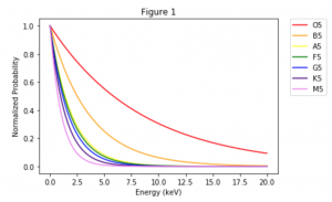
Stars produce immense amounts of energy every second, thanks to quantum tunneling. There is no comprehensive classical approach to explaining how fusion could occur in stellar cores due to the Coulomb barrier; but very small, nonzero, probabilities of two protons tunneling does. To determine fusion reaction rates inside of stars, we have to consider two probabilities: 1) the probability of a given particle having a certain energy and 2) the probability of a particle tunneling at a certain energy. Assuming a Maxwellian distribution of energies, these two work against each other in the way that there are less available particles with increasing energy, but higher energy particles have a higher probability of tunneling through the Coulomb barrier. For a given spectral type (since we have a given temperature), we can multiply these two probabilities to obtain a final curve that will have a peak known as the Gamow Peak. The area under the Gamow peak determines the reaction rate!

Maxwellian Distribution

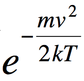
The Maxwellian distribution can be found by the following probability:

Source: http://astro1.physics.utoledo.edu/~megeath/ph6820/lecture26_ph6820.pdf

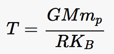
where k is the Boltzmann constant, T is temperature, and {(mv^2)/2} is the kinetic energy. We know the value of k, 8.61733e-8 keV/K, and will vary energy; so all that is left to be determined is temperature. While I found accessible values for stellar surface temperature I needed to calculate stellar core temperatures, as that is the site of nuclear fusion. We can find an equation for stellar core temperature by equating the force due to pressure gradient to the gravitational force to obtain:where G is the gravitational constant, M is the mass of the star, m_p is the mass of a proton, R is the radius of the star, and K_B is again, the Boltzmann constant. With this, I calculate that:

From this, I can plot the Maxwellian distributions:

Tunneling Distribution

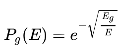
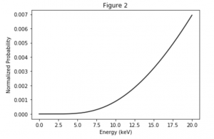
We can find a single probability curve for quantum tunneling that we can apply to all spectral types since it is independent of temperature. For two nuclear particles to overcome the electrostatic potential, physicist George Gamow found that the probability is:

where E_g is the Gamow energy, given by:

where m_r is the reduced mass of the two particles, c is the speed of light, alpha is the fine structure constant, Z_a and Z_b are the respective atomic numbers of each particle. The last two are equal to 1, since I am only considering at the first step of the proton-proton chain. I find the following:

Gamow Peak

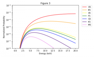
From here, I will multiply the Maxwellian distribution of particles for each spectral type by the probability distribution of tunneling. When multiplied together, the function produced represents the probability density function of quantum tunneling given a distribution of particles that have various speeds and thus various energies. The peak of this pdf is called the Gamow Peak. The area under the Gamow Peak determines the reaction rate! I find the following:

Above is a plot of all the reaction probabilities for each spectral type. Since the luminosity axis of the H-R diagram is logarithmic, our dispersion in temperature is logarithmic, so I thought it would be a bit more useful to display the same plot from Figure 3, with a logarithmic y-axis. It can be seen that the Gamow Peak increases as temperature increases with spectral type, from the coldest stars at M5, to the hottest stars at O5. This indicates that the reaction rates will increase with increasing core temperature, which makes intuitive sense. However, it is more difficult to see a distinct “peak” from the curves of the really hot O5 and B5 stars, due to the increased energy in these cores. The effect of this is that fusion for heavier atoms through the CNO process actually dominates rather than the proton-proton fusion that dominates cooler stars like our Sun. Still, the reaction rates for proton-proton fusion are much higher for hotter stars.

References

Link to Code

I did all of my work in a Jupyter notebook using Python. It is annotated so that hopefully one can follow along with the code:

PHYS 320 Project

Escape the Potential: A Quantum Mechanics Board Game

Overview:

Escape the Potential is an educational game that I designed with Aidan. The main goal of this game is introduce quantum mechanics concepts to high school students with a background in physics. It could also be used as a review for college level students. While Aidan focused more on the logistical side of designing the game, I focused more on the pedagogy.

How to Play:

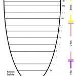
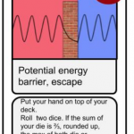
This game is for 2-4 players and the goal is to ‘escape’ the potential well. There are three different potential well boards you can choose to play with; infinite square well, finite square well, harmonic oscillator well (shown below).

: finite square well

: SHO well

: infinite square well

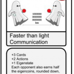
Each player starts with three cards in their hand. Players take turns playing their hand and earning eigencoins as they move up eigenstates in the potential well. Once a player has earned eigencoins, they can choose to save them or to purchase new cards (shown below).

: angular momentum

: blackbody radiation

: CERN

: entanglement

: Fabiola Gianotti

: hydrogen

: Lene Hau

: lowering operator

: Maria Goeppert-Mayer

: normalize

: photoelectric effect

: raising operator

: schrodinger’s cat

: spooky action at a distance

: tunneling

: Vera Rubin

: wavefunction

Before they can purchase the new card though, they must learn about the card using the card appendix. Over the course of the game, players purchase enough cards that they are able to escape or tunnel out of the well at the end of their turn.

The complete set of rules are here.

How to Teach:

This game is simple to implement as a teacher. The thing the teacher should focus on is answering student questions and making sure the class is engaged. I created a potential lesson plan a high school physics teacher could use in the classroom. It would be an ideal game to play at the end of the school year after students have been familiarized with classical physics concepts.

I based the pedagogy of this game and the lesson plan off of three main ideas:

Focus should be more on interpretations of quantum mechanics than on calculations. [1]
Emphasis should be placed on the difference between the quantum concepts students are learning and the classical concepts they are familiar with. [2]
It should be made clear that quantum physics is probabilistic and not deterministic. [3]

By teachers putting the spotlight on interpretations of quantum physics, students will be able to grasp the concepts instead of struggling with the complicated calculations. After playing this game, I want students to have a greater appreciation for the world and a broader understanding of what physics is and how it applies to them.

My Experience:

Making this game forced me to really make sure I knew the basics of quantum mechanics. Additionally, I got to learn about a range of complicated, fascinating quantum phenomena like quantum entanglement and action at a distance. I like making lessons plans, and it was nice to see my vision for the game evolve and come together in the end. I wanted to create a fun and interactive way for high school students to get their first taste of quantum physics. After the initial struggle of coming up with what type of game we wanted to create and what we wanted students to get from it, the entire process was rewarding and fun. It was just a matter of researching, creating, playing, and revising our game.

Escape the Potential would not have been the same if it hadn’t been for Aidan. He was very detailed oriented and on top of creating the foundations for our game. I enjoyed getting to be creative and applying some of what I’ve learned in my education courses to my physics course. Overall, my experience was positive and I grew from it.

Our game is available to play in Sanders Physics 201.1.

: Not included in the picture are the “Eigencoins” used as currency in the game. They are large silver coins.

References:

All images are from Wikimedia and are available for use under the (insert link for creative commons).

[1] . C. Baily and N. D. Finkelstein, “Teaching and understanding of quantum interpretations in modern physics courses,” American Journal of Physics (January 2010). https://doi.org/10.1103/PhysRevSTPER.6.010101

[2] R. Müller and H. Wiesner, “Teaching quantum mechanics on an introductory level,” American Journal of Physics (March 2002) https://www.tu-braunschweig.de/Medien-DB/ifdn-physik/ajp.pdf

[3] K. Krijtenburg-Lewerissa, H. J. Pol, A. Brinkman, and W. R. van Joolingen, “Insights into teaching quantum mechanics in secondary and lower undergraduate education,” American Physical Society (February 2017) https://doi.org/10.1103/PhysRevPhysEducRes.13.010109

Fundamental Rovibrational Spectrum of CO

Motivations

Protoplanetary disks are regions of planet formation around young stellar objects. Astronomers observe these regions to get snapshots of the planet formation process. Protoplanetary disks are optically thick at visible wavelengths, meaning that photons in the visible part of the electromagnetic spectrum from the star are absorbed by the disk and do not reach observers on Earth. Millimeter wavelength light is not absorbed by the disk as much, and so by observing light in that range, astronomers can learn about the morphology of disks. One key molecule abundant in protoplanetary disks is carbon monoxide (CO). Because of the low temperatures of disks (around 40 K), the energy transitions observed fall in the rotational and vibrational (rovibrational) regime.

Overview

When two atoms form a stable covalent bond, they can be thought of semi-classically as a two atoms connected by a spring. That spring can vibrate, and the energies of the vibrations can be found by treating the bond as a harmonic oscillator. This gives us

where v is the vibrational quantum number associated with different vibrational energy levels.

Diatomic molecules can also rotate in different ways, corresponding to different rotational energy levels. Assume that the molecules act as rigid rotors, meaning you assume that the molecules are connected by a solid rod as they rotate so that the bond length does not change. This lets you solve the Schrödinger equation and get the allowed energies.The energy associated with a rotational state is given as

where j is the rotational quantum number and I is the moment of inertia of the molecule. Molecular spectroscopists define the rotational constant B

which has which as units of energy. B changes based on the molecule, and for CO I found the value of B to be as listed above.

My goal with this project was to explore the fundamental rovibrational spectrum of CO. I first investigated energy in a rovibrational system and plotted how it changes for different rotational states. I did this using Python 3 and the libraries NumPy and Matplotlib. Then I modeled the intensity of different lines in the fundamental spectrum of CO and overlaid it with experimental data taken from the high-resolution molecular absorption database (HITRAN).

Selection Rules

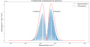
Selection rules describe what quantum state transitions are allowed in a given system. The fundamental spectrum in this context refers to the transition in which the vibrational state (v) changes by +- 1. This gives rise to the selection rules. If the vibrational state changes by +- 1, the rotational state must also change by +- 1, no more and no less. In this field, the [forbidden] transition of Δv = +- 1 and Δj = 0 is called the “Q branch”, and it appears in Fig. 3 as an empty spot in the middle. When the rotational state changes by +1, the transition is said to be in the “R branch”, and when it changes by -1 the transition is in the “P branch”. These selection rules can be summarized as:

Both the vibrational and rotational quantum numbers must change
Energy of rotation can be added to (in the R branch) or subtracted from (in the P branch)

The energy of transitions in the R and P branches respectively are:

where the first term corresponds to initial energy of the system before the transition.

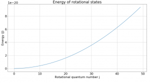
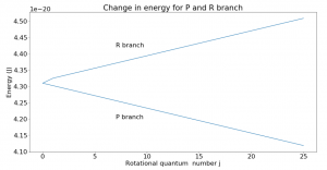
Though the energy of rotational states increases with increasing j, the difference between two consecutive levels is always 2B, where B is the rotational constant. This can be seen in Fig. 2. If going to a higher rotational state (in the R branch), add 2B to get the new energy level; subtract 2B for a lower state.

Results

Fig. 1

Fig. 1 shows how rotational states increase in energy based on the equation listed above. Despite the slope of this graph not being constant, a look at the change in energy between levels reveals an interesting fact about rotational transitions.

A constant slope means changes in energy are equal

Fig. 2

Fig. 2 plots change in energy vs. rotational quantum number for the R and P branches. The Q branch is the corner point where no transitions occur. From the graph, we can see that if undergoing a transition on the R branch, the energy of the state will increase linearly from one state to the next. That change is given by the slope of the graph which was found to be 2B, as expected. Similarly, the P branch energy transitions decrease by 2B from one transition to the next. Note that the rotational quantum number j can only increase or decrease by 1 with each transition.

Theoretical and experimental rovibrational CO

Fig. 3

Fig. 3 plots the theoretical relative intensities of different transitions based on the following equation:

where k is the Boltzmann constant and the temperature T was set to 300 K. The blue spectral lines come from experimental data from HITRAN. The x axis is given in wavenumbers, a unit commonly used in molecular spectroscopy.

Discussion

Fig. 3 was the most challenging result for me to produce and took several weeks of trying many different methods. Plotting the actual data was somewhat simple with Python, but calculating the relative intensities took me down many dead ends before finally getting the end result. Different sources listed different equations for intensity and different values of B. Eventually after calculating my own B and using an equation from Bernath, I was able to get the desired result.

I expected that the theoretical and experimental distributions would not match exactly, and that is because real molecules do not act exactly like rigid rotors. They experience centrifugal distortion and rovibrational coupling, which both add complications to the simplistic energy equations I used. However, my goal was to calculate the simplistic version of the fundamental rovibrational spectrum, and I accomplished that. In future work I would like to try to add complications to the model to better fit real data. I would also like to see how the environment of a protoplanetary disk could affect the spectrum.

References

Spectrum of Atoms and Molecules by Peter F. Bernath

Fundamentals of Molecular Spectroscopy by C. N. Banwell

Chemistry LibreTexts

SpectralCalc

HITRAN

Observing Quantum Entanglement Through Spontaneous Parametric Downconversion

In this project, I (and partner Jay Chittidi) investigate the concept of quantum entanglement in an experimental context. I will show how entanglement not only relates to the concept of superposition but also how it furthers our understanding of the differences between the laws of Quantum Mechanics and Classical Physics.

What is Quantum Entanglement?

Entangled particles are in a special kind of superposition of states such that either of their wavefunctions cannot be considered independently from the other. In other words, a measurement on one of the particles instantly affects that of the other.

To illustrate how an entangled state differs from a simple superposition of two states, we can consider two photons that have two corresponding polarization states, horizontal or vertical. A non-entangled state for each photon would look like the following:

[1]

In this case, each photon is in a superposition of vertical and horizontal polarization and the coefficients A,B,C, and D represent the probability of measuring vertical or horizontal for each photon.

If the photons were in an entangled state, their wavefunctions could look something like this:

[2]

In this case, both the photons have the same wavefunction, which depends on the horizontal/vertical polarization state of either photon. This means that any measurement of one photon will depend on the measurement of the other. Note that there are multiple ways to achieve this; the equation above is just one example.

To illustrate this further, we can calculate the expectation value of some measurement, by assuming there exists some hermitian operator, O, for this measurement:

If the photons were not entangled:

[3]

If the photons were entangled,

[4]

Equation 3 shows that the non-entangled photon has an expectation value for the measurement that only depends on its own polarization state. In contrast, equation 4 shows that this expectation value for an entangled particle depends on the polarization states of both particles. Thus, at the time of the measurement, both particles will instantaneously collapse into corresponding states.

Hidden Variable Theory

We can also examine entanglement through the lens of hidden variable theory. As stated above, when one measurement is taken from a member of an entangled pair, the other one instantaneously collapses into a corresponding state based on their mutually dependent wavefunction. Even if the photons are on opposite ends of the universe, this collapsing effect would theoretically be the same. If the wavefunctions collapse instantaneously even at astronomical distances, then information needs to travel faster than the speed of light. One explanation for this “magical” phenomenon is that there exist hidden variables that predetermine the outcome of each measurement before it occurs.

In 1969, Clauser, Horne, Shimony, and Hotle (CHSH) created a generalized hidden variable theory which they used to derive an inequality that would only be true if hidden variables are at play in a given measurement. [2] They did this by assuming the outcome of a given measurement depends on the independent parameters involved and some arbitrary “hidden variable” in some way. Then, they derive an expression, Bell’s inequality, which will always be true for a given set of measurements if hidden variables are involved. The derivation of this inequality is not trivial and purely mathematical, so it is not relevant to this project. They also proposed an experiment to test their inequality that consists of measuring the number of coincident photons as a function of polarization of either photon. If we can prove that no hidden variables exist, then we will show that the behavior of entangled particles contradicts our understanding of classical physics.

Testing Quantum Entanglement Experimentally

To conduct our entanglement experiment, we utilized the phenomenon of spontaneous parametric down-conversion (SPDC). SPDC occurs when light passes through a nonlinear crystal (in our case BBO). A small number of photons that pass through the crystal split into two photons with equal energy that is half that of the incoming photons. They also have the same polarization that is orthogonal to the polarization of the incident photon due to conservation of angular momentum. In our experiment, we sent a purple laser first through a half-wave plate to polarize the laser light at 45 degrees. The polarized laser light then passed through two BBO crystals oriented perpendicular to each other. This means that the down-converted photons could either be horizontally or vertically polarized, but since we can’t predict which crystal produced the pair, we don’t know their polarization. This phenomenon causes the photons to be in an entangled state, where the measured polarization of one photon depends on that of the other. If the photons were not entangled, they would be in a randomly mixed state of horizontal and vertical polarization, whereas entangled photon pairs would have correlated polarizations.

The following formulas define variables, E and S, which don’t have a physical meaning. These formulas are just CSHC’s original hidden variable theory rearranged in a more convenient manner.[1][3]

[5]

[6]

In these formulas, N is the number of coincidences recorded for the given combination of polarizer angles. Theta1 and theta1 prime are any two polarization and angles for detector A and theta2 and theta2 prime are any two polarization angles for detector B. Based on the work of CHSH S ≤ 2 if hidden variables are involved in the measurement of coincidences.[1][3] Thus, the expected results of our experiment would be an S that is greater than 2.

Experimental Procedure

Figures 1 and 2 show our experimental setup. The laser is shot through the half-wave plate, the BBO crystals, and also a quartz that corrects for the phase shift of the laser light.

We can see that the two detectors on the other side of the optical table are approximately equidistant from the principle beam in order to detect the two streams of down-converted photons. There is a polarizer in front of each detector in order for us to test the CHSH hidden variable theory. We also placed infrared filters in front of each detector so that they would only detect the stream of infrared photons.

Figure 1: Birds-eye view of experimental setup

Figure 1: Close up of detectors with polarizers in front

We used a LabView program (made by previous Vassar students) to record the total number of coincidences in each a 10 second interval. A coincidence is recorded every time the detectors register a photon instantaneously. Since the down-converted photons are in an entangled polarization state and have correlated polarization, the number of coincidences is a function of polarizer angle. The number of coincidences is also the measurement needed to verify equations 5 and 6.

Since S depends on configurations independent calculation of E, and each calculation of E depends on the number of coincidences at four polarizer configurations, we needed to measure the number of coincidences at 16 polarizer configurations in total.

Results and Conclusions

Table 1 shows the results of our experiment. The number of coincidences is clearly a function of polarizer angle, which indicates that the photons are in fact in an entangled state.

Table 1: Coincidence counts and total counts in each detector at each of the 16 combinations of polarizer angles. The first two columns show the angle of each polarizer. The third column shows the counts in detector A, the fourth shows the counts in detector B, and the fifth shows the coincidence counts.

Our final value of S, using equations 5 and 6 was -0.0465±0.0396. Unfortunately, this obeys Bell’s inequality for hidden variables, which is the opposite of what we had expected. We know from many previous repetitions of this experiment at other institutions, that Bell’s inequality should not hold in this experiment.[1][3] The uncertainty in our value of S is also about the same as the calculated value itself, so we are not very confident in our result.

There are various sources of error that could have resulted in the data we collected. There could have been some sort of light pollution that we weren’t accounting for or some hardware error. However, since our experimental setup has been extensively tested by previous students, these effects probably weren’t significant enough for us to get such an inaccurate value of S.

The most likely cause of the discrepancy between our data and the CHSH theory is improper alignment. Most of our time working on this project was spent attempting to align the laser. We struggled not only to align the detector with the beam infrared photons, but also to maximize the coincidences. For a more detailed description of our struggles, see Jay’s project.

From comparing our data to the data collected by Dehlinger and Mitchell using a similar experimental setup[1], we have deduced that at a given polarizer angle for detector A, the number of coincidences should vary sinusoidally with the polarizer angle for detector B. Figure 3 shows that at the different values of angle for polarizer A, the number of coincidences does not vary in this fashion with the angle for polarizer B. We think that we could solve this issue by aligning the two detectors more thoroughly. The down-converted photons are actually emitted in ring, where photons across from each other are entangled pairs (illustrated in Figure 4). This means that if our detectors weren’t on the exact spots on the ring that correspond to an entangled pair, our data would not necessarily be consistent with CHSH theory or previous results. For future research, if we were able to place both detectors in some sort of circular mount with adjustable positions, then we would be able to more easily identify these exact positions. We also began our experiment with detector A already aligned and proceeded to align detector B. It is possible that we would have needed to align detector A more exactly in order to locate the correct ring positions.

Figure 4: Number of coincidences as a function of polarizer angle for detector B (beta) at different values of polarizer angle for detector A (alpha).

Figure 5: Schematic of SPDC. The entangled pairs are emitted in all orientations but at the same angle. They end up emerging from the BBO crystal in a ring shape, with entangled pairs exactly across from each other.

Regardless of some clear experimental issues, we were able to observe quantum entanglement in action. Although the number of coincidences we recorded did not show the correct dependance on polarizer angle, they displayed a clear relationship. This is a clear indicator that when one member of an entangled pair is counted, the other must instantaneously collapse into a corresponding polarization state to be counted by the other detector. And although we did not end up disproving CHSH’s hidden variable theory, our calculation of S came with an unreasonable uncertainty, so our results cannot prove that hidden variables exist. Inconclusive results aside, this project was very useful in illustrating the concepts of quantum entanglement and hidden variables, which relate to the most fundamental concepts of quantum mechanics such as superposition and deviation from classical mechanics. If anything, this experiment allows us to observe the oddity of quantum mechanics by simply counting photons.

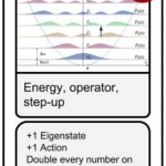
References

[1] Dehlinger, Dietrich and Mitchell, M.W. “Entangled photons, nonlocality and Bell inequalities in the undergraduate laboratory.” American Journal of Physics 70, 903 (2002).

[2] John F. Clauser, Michael A. Horne, Abner Shimony, and Richard A. Holt. “Proposed Experiment to Test Local Hidden-Variable Theories” Physics Review Letters 23, 880 (1969).

[3] Galvez, Enrique J. “Correlated Photon Experiments for Undergraduate Labs” Colgate University (2010).

Background:

The Selection Rules

The Laporte Selection Rule

Two even states:

Two odd states:

One even and one odd state:

Spin Selection Rule

Singlet to Triplet Transition

Zeeman Effect

Franck-Condon Principle

Overlap of Zero-zero transition S00

Overlap of S01 Transition

Applicational Experiment: Photobleaching of Methylene Blue

Experimental Background:

Experimental Procedure and Results:

By Jay Chittidi (’19), Lab Partner: Ellis Thompson (’20)

Warming Up to Entanglement

Our Experimental Setup and More Background

Figure 1: A bird’s eye view of the stage. See above for a detailed description

Figure 2: The detector assembly. Detector B is on an XYZ Transform to aid in alignment. See below for more details.

Figure 3: A diagram in a semi-2D plane of the ring of down-converted photons. Note that the purple beam is exactly in the center of the cone.

Our Struggles

Data

Results

Conclusions

Acknowledgements

References

Motivations

Overview

Selection Rules

Results

Discussion

References

What is Quantum Entanglement?

[1]

[2]

[3]

[4]

Hidden Variable Theory

Testing Quantum Entanglement Experimentally

[5]

[6]

Experimental Procedure

Figure 1: Birds-eye view of experimental setup

Figure 1: Close up of detectors with polarizers in front

Results and Conclusions

Figure 4: Number of coincidences as a function of polarizer angle for detector B (beta) at different values of polarizer angle for detector A (alpha).

Figure 5: Schematic of SPDC. The entangled pairs are emitted in all orientations but at the same angle. They end up emerging from the BBO crystal in a ring shape, with entangled pairs exactly across from each other.

Overlap of Zero-zero transition S₀₀

Overlap of S₀₁Transition