Category Archives: Advanced EM

Advanced Electromagentism (Phys 341)

Phase Modulation

Phase modulation is not a very difficult concept to grasp. In my blog proposal I presented this equation

(1)   \begin{equation*} \frac{1}{n^{2}}=\frac{1}{{n_{0}}^{2}}}+rE+RE^2 \end{equation*}

This allows you to change the index of refraction with an applied electric field. The speed a wave travels inside a new medium is equal to the speed of light in a vacuum divided by the index of refraction of the material v=\frac{c}{n}. Using this relationship and the equation above, we have an expression that relates the applied electric field strength to the speed of the wave in inside the crystal.

(2)   \begin{equation*} {v^{2}}=\frac{c^{2}}{{n_{0}}^{2}}}+rEc^2+RE^2{c^2} \end{equation*}

Once the wave exits the EoM it will have a shift in phase. Being able to vary the speed of the laser inside the crystal very slightly will give you the ability to modulate the phase of the laser so that you can have it exit the EoM at what ever point in its oscillation you wish.

Here is an animation showing a light wave entering a crystal and slowing down having its phase shifted. I could not figure out how to draw lines on the graph but the crystal is from 0 to 2\pi

.

Share

Jones Vectors and Matrices

I think it is important to have an introduction into Jones vectors and matrices. A Jones vector is when you represent the Electric field as such

(1)   \begin{equation*} \vec{E}}=\begin{bmatrix} E_{x}\\E_{y} \end{bmatrix} \end{equation*}

A Jones matrix is a 2 by 2 matrix that does some kind of operation on the Jones vector thereby transforming it. These Jones matrices vary depending on the optical element that your electromagnetic wave is traveling through. Some examples of Jones matrices

Horizontal Polarizer:

\begin{vmatrix} 1 & 0\\ 0& 0 \end{vmatrix}\rightarrow \begin{bmatrix} 1 & 0\\ 0& 0 \end{bmatrix}\begin{bmatrix} E_{x}\\ E_{y}  \end{bmatrix}=\begin{bmatrix} E_{x}\\ 0  \end{bmatrix}

Vertical Polorizer:

\begin{vmatrix} 0 & 0\\ 0& 1 \end{vmatrix}\rightarrow \begin{bmatrix} 0 & 0\\ 0& 1 \end{bmatrix}\begin{bmatrix} E_{x}\\ E_{y}  \end{bmatrix}=\begin{bmatrix} 0\\E_{y} \end{bmatrix}

Half wave plate:

\begin{vmatrix} cos2\theta & sin2\theta\\ sin2\theta& -cos2\theta \end{vmatrix}\rightarrow \begin{bmatrix} cos2\theta & sin2\theta\\ sin2\theta& -cos2\theta \end{bmatrix}\begin{bmatrix} E_{x}\\ E_{y}  \end{bmatrix}=\begin{bmatrix} E_{x}cos2\theta+E_{y}sin2\theta\\E_{x}sin2\theta-E_{y}cos2\theta  \end{bmatrix}

\theta is the angle that the half wave plate is oriented at. These Jones vectors will be useful in describing how the electromagnetic wave is polarized in the following posts

Share

Electromagnetic Waves

Before I go into any detail of the modulation of laser beams I think it is important to mention that you can obtain the full expression of an electromagnetic wave through just knowing how the electric field is behaving. The electric field is related to the magnetic field by

(1)   \begin{equation*} \vec{B}=\frac{1}{c}\hat{k}\times\vec{E} \end{equation*}

Where \hat{k} is the unit vector pointing in the direction of propagation.From this point on I will only talk about how the electric field is behaving.

Share

Derivation of my Modeling Equation: version 1.5

Below is my updated equation that I will use to model the emf produced by my induction generator, as well as the derivation that led me to it.  The objective of my work and the variables dealt with remain the same as in my last post, this is more meant to expose the inner workings of how I came up with the equations that I did.  The majority of the information here comes from common sense equations (d = rt, for example).  The only more complicated equations thatI am using are Griffiths 7.13: relating emf to change in flux, and the expression for the Fourier Transform of a triangle wave, taken from Wolfram Mathworld.  Now, on to the derivation.

We look at a cylindrical rotor of radius $a$ contained within a cylindrical stator of radius $b$, with $n$ coils of wire of length $l$ and width $w=\frac{2 \pi b}{n}$.  The height of the wire coil is irrelevant as it is directly proportional to the number of coils, which we will not be dealing with.

We begin by looking at the flux through a single loop, assuming $\vec{B}$ is parallel to the normal vector $d\vec{a}$.

    \[\Phi = \int \vec{B} \cdot d\vec{a} = BA_{loop} = Blw = Bl\frac{2 \pi b}{n}.\]

Simple enough.  Now we only have to find $B$.  As we know that magnetic field strength varies as the inverse cube of the distance from a magnet, we can first say that

    \[B = \frac{1}{r^3} B_0 = \frac{B_0}{(b-a)^3}\]

,

$B_0$ being the magnetic field strength of the magnet.  We also know that flux changes with time periodically, and linearly.  A sine wave seeming inappropriate even as an approximation in this case, we use the Fourier Transform of a triangle wave to approximate.  This gives us

    \[B = \frac{B_0}{(b-a)^3}   [\frac{8}{\pi ^2} \Sigma_{k = 1, 3, 5}^{\infty}   \frac{(-1)^{(k-1)/2}}{k^2}   \sin(fkt)]\]

where $f$ is the frequency with which a coil undergoes a full cycle between North and South magnetic fields (ie, the time that it takes for a North and South magnet to pass by the coil).  To make this a bit simpler to think about, we imagine the period $T$.

    \[T = \frac{\text{angle passed through}}{\text{velocity with which magnets pass through angle}} = \frac{2 \cdot (2 \pi / n)}{\omega_s - \omega_r} = \frac{4 \pi}{n(\omega_s - \omega_r)}\]

where $\omega_s$ and $\omega_r$ are the rotation frequencies of the stator and the rotor, respectively.  From here, it follows that

    \[f = \frac{1}{T} = \frac{n(\omega_s - \omega_r)}{4 \pi}\]

..

With this in mind, we proceed to the next step of our approximation, leaving $f$ in for the sake of simplicity.  We now approximate the Fourier Series with the first three terms, and multiply by our previously established area to give us magnetic flux through a loop.

    \[\Phi = \frac{16B_0b}{(b-a)^3n \pi} [\sin(ft) -\frac{1}{9}\sin(3ft) + \frac{1}{25}\sin(5ft)]\]

.

Finally, we take the time derivative of this expression and multiply by a negative n to give us the emf induced in every coil in the stator as the rotor spins.

    \[\varepsilon = -\frac{4B_0bn(\omega_s - \omega_r)}{(b-a)^3\pi ^2} [\cos(ft) - \frac{1}{3}\cos(3ft) + - \frac{1}{5}\cos(5ft)]\]

with

    \[f = \frac{n(\omega_s - \omega_r)}{4 \pi}\]

.

Share

Scattering-Preliminary Results

Graph of Predicted Scattering Intensity vs. Wavelength (for different particle concentrations)

Equation [3] was used in order to predict the scattering intensity as a function of wavelength (within the visible spectrum) for different volumes, or concentrations, of particles.

The diameter of the particle used to create this graph was 105 nm.  In order to determine the refractive index of the particles used I looked at the refractive index of polylatex microspheres that I have previously worked with in the VAOL lab.  The refractive index of these microspheres was 1.59.  The refractive index of water is 1.33.  The length of the cuvette was also determined from previous lab work and was approximately 1 cm.  The incident intensity was also taken from experimental data and the value used was 0.365 Volts.  The volume of particles used ranged from a “dropsize” of 20 microliters to 45 microliters in 5 microliter increments.

As shown in the graph above, the predicted scattering intensity increasing as concentration of the particles increases.  This makes sense because as the number of particles in the cuvette increases show does the chance that the light will interact with a particle(s) resulting in more scattering.   From this graph it also appears that light is scattered more (at 90 degree side scattering) for shorter wavelengths.  This result is consistent with Rayleigh theory.  (And also explains why the sky is blue!  Longer wavelengths mostly pass right through the atmosphere, but shorter wavelengths–like blue light–are scattered in every direction.  So no matter what direction you look some scattered blue light reaches your eyes!)

Polar Plot depicting the Rayleigh Relative Scattering Intensity for scattering angles from 0 to 360 degrees as Particle Size increased (for wavelengths within the visible spectrum and particles within the Rayleigh limit)

The color of the plot shows the color of the light (wavelength) used.  The particle sizes used depended on the wavelength of light used (since Rayleigh scattering is wavelength dependent and for longer wavelengths larger particles can be used within the Rayleigh limit).  A volume of 200 microliters was used.  The cuvette length, incident intensity, refractive index of the particle, and the refractive index of water were all kept the same as for the graph above.

The graph (below) is a composite image of the polar plots for the different wavelengths (above).

These graphs show that larger particles scatter more light.  That is why the purple and blue  wavelengths have such a small scattering intensity when compared with the orange and red, even though purple and blue wavelengths should be scattered more.  The particle sizes for these wavelengths, however, had to be smaller than for red or orange because Rayleigh scattering is wavelength dependent and can only accurately predict scattering intensities for particles less than one-tenth the wavelength of light.

Since the graph above can be misleading because it may make it appear that longer wavelengths (like red) are scattered more than shorter wavelengths (like purple) for Rayleigh scattering, even though (as I said above) the reason is due to particle size and the Rayleigh limit being larger for longer wavelength, I’ve included a graphs (below) of Rayleigh scattering that are identical to graphs above except the particle sizes were held constant for all the wavelengths.

These graphs show that for Rayleigh scattering shorter wavelengths are scattered more than longer wavelengths and that larger particles produce more scattering.

Polar Plot depicting the Rayleigh-Debye Relative Scattering Intensity for scattering angles from 0 to 360 degrees as Particle Size increased (for wavelengths within the visible spectrum and particles greater than the Rayleigh limit)

The color of the plot shows the color of the light (wavelength) used.  The particle sizes used were the same for every wavelength.  The size ranged from 100 to 200 nanometers in increments of 10 nanometers.  A volume of 200 microliters was used.  The cuvette length, incident intensity, refractive index of the particle, and the refractive index of water were all kept the same.

The graph (below) is a composite image of the polar plots for the different wavelengths (above).

These graphs show that shorter wavelengths scatter more light (as expected) when the particle size range for each wavelength is identical.  These graphs also show that for Rayleigh-Debye scattering most of the light is scattered in the forward direction.

Share

revised project plan

For my project I will be examining the effect of varying coil numbers, distances between stator and rotor, resistance of the wires involved, and relative frequencies of rotation of the stator and rotor on the induced current in the coils, and thus the power provided to the grid.

To derive the equation that I will be using for my model I have made several simplifying assumptions, including that the coils, the rotor, and the stator all have the same length, that coils and magnets are squares that pass straight by each other, and that the strength of the magnetic field passing through a given coil as the magnet moves by is sinusoidal.  The equation that I have derived is below.

Share

Project Proposal 2

For my project I will attempt to model the magnetic field from a magnet as it interacts with a wire coil. I will make an interactive model that can vary speed, distance of coil to magnet, magnet intensity, and number of turns among other things. My first attempt at the animation can be seen below.

And here it is to illustrate the movement:


As is evident by this picture, I still have yet to add the magnetic field lines, and that is where the bulk of my project will be. I will be using our Griffiths textbook, The Art of Electronics by Horowitz & Hill, The Handbook of Tables for Applied Engineering Science, and Engineering Circuit Analysis by Hayt and Kemmerly. I also have collected a few journal volumes that I will use as I see which are the most useful.

I will be using the equation

(1)   \begin{equation*} B=\frac{\mu _{0}2\mu^{2}}{4\Pi d^{3}} \end{equation*}

as well as

(2)   \begin{equation*} \Phi ^{_{B}}=Ba \end{equation*}

   and  

(3)   \begin{equation*}     \epsilon =-n\frac{d\Phi _{B}}{dt}   \end{equation*}

Where \mu 
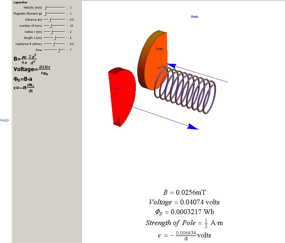
is the Magnetic Moment, \epsilon is the electromotive force, and \Phi^{_{B}}

Since I will have the magnet moving over a stationary wire coil, we will see that electric fields (not magnetic forces) are responsible for setting up the emf. Although the electric and magnetic fields are inextricable linked, it is useful to note that because stationary charges can’t experience magnetic forces, there has to be another explanation.


The unanswered question is how to mathematically model the magnetic field due to these magnets. I currently will be simplifying each magnet to a magnetic dipole, as opposed to a more complex magnet.  I would hope to have their intensities change as I change the magnetic moment, and I would also like to see what kind of feedback the solenoid would produce. In order to simplify this process the next iteration of my animation will be a square magnet and a square coil. This should hopefully make the modeling easier, as their seems to be more information on that kind of a set-up.


Share

Project Plan

My project will explore the effect of varying slip, rotation frequencies, and system size/configuration on the energy output of an induction generator.  If time and resources permit, I will also be testing how efficiency varies with slip, and how this effects my final results of which configuration is best.  This question (of bigger versus smaller systems with higher or lower rotation frequencies) is currently a topic of much debate in the field of wind turbine design, and thus is an interesting area to conduct my research.

The traditional design for an induction generator includes a gearbox with which to convert the relatively slow rotor rotations provided by the mechanical source (wind, steam, etc.) into rotations at a frequency that will generate power.  However, a newer model forgoes this for a much larger ring of permanent magnets, creating a stronger magnetic field that does not require the rapid rotation rate provided by the gearbox to generate a sufficient amount of power.  The basic equations that will form the backbone of my simulations are described below.

I will apply these equations to relate slip and the relative size, position, and number of loops of wire to the amount of current generated, and run simulations to find the most efficient configuration.


Share

Project Plan

Second Harmonic Generation is a special case of optical mixing. It is a process by which photons from a laser beam are mixed in a nonlinear medium and the output photon has double the energy and frequency and half the wavelength. Conditions satisfy $\omega_{1}=\omega_{2}=\omega$ and $\omega_{3}=2\omega$. Both energy and momentum conservation must be satisfied. Energy by $\omega_{3}=\omega_{1}=\omega_{2}$ and momentum by $k_{3}=k_{1}+ k_{2}$

In more detail:
“Nonlinear optics is the study of phenomena that occur as a consequence of the modification of the optical properties of a material system by the presence of light”. Input waves are at frequencies $\omega_{1}$ and $\omega_{2}$. By the nonlinear effects of incident beams (at the atomic level) each atom develops an oscillating dipole moment which contains a component at frequency $\omega_{1}+\omega_{2}$. Each atom radiates this frequency but there are many atoms in our medium and hence many atomic dipoles oscillating with a phase determined by the phases of the incident waves. When the relative phasing matches the waves radiated by each dipole will add constructively turning the system into a phased array of dipoles. When this happens the electric field strength of the radiation emitted will be the number of atoms times larger and hence the intensity will be the number of atoms squared.

I will assume my system to be lossless and dispersion-less for simplifying equations

(1)   \begin{equation*} \bigtriangledown \times \bigtriangledown \times \widetilde{E}_{n} + \frac{\epsilon^{(1)}(\omega_{n})}{c^{2}} \bullet \frac{\partial^2 \widetilde{E}_{n}}{\partial t^2} = \frac{-4\pi}{c^2} \frac{\partial^2 \widetilde{P}^{NL}_{n}}{\partial t^2} \end{equation*}

2.1.19 Nonlinear optics Robert W.Boyd

$\widetilde{P}^{NL}_{n} =$ Non-Linear part of Polarization Vector

$ \widetilde{E}_{n} =$ Electric Field vector

$\epsilon^{(1)}(\omega_{n}) =$ Frequency dependent dielectric Tensor

Equation (1) is derived from Maxwell’s equation and is the equation for waves in medium. It is valid for each frequency component of the field.

$\widetilde{E}_{2}(z,t) =A_{2}e^{i(k_{2}z-wt)},   \widetilde{P}_{j}(z,t) =P_{j}e^{-i\omega_{j}t},$    $P_{1} =4dA_{2}A^{*}_{1}e^{i(k_{2}-k_{1})z}, P_{2} =2dA^{2}_{1}e^{i2k_{1}z}$

2.2.1, 2.2.3, 2.2.4,2.2.5, 2.2.7  Nonlinear optics Robert W.Boyd

$\widetilde{E}_{2}(z,t)$ will be my equation for the transmitted wave at frequency  propagating in the z direction,$ \widetilde{P}_{2}(z,t)$ the nonlinear source term and $P_{2}, P_{1}$  the amplitude of the nonlinear polarization and amplitude of incident beam respectively. I will make diagrams of incident waves hitting the medium and resulting transmitted wave.

Substituting the transmitted wave equation in the wave equation and solving by hand I will find coupled amplitude equation.

(2)   \begin{equation*} \frac{dA_{2}}{dz}= \frac{4 \pi id \omega^{2}_{2}}{k_{2}c^{2}}A^{2}_{1}e^{i\bigtriangleup kz} \end{equation*}

2.6.11 Nonlinear optics Robert W.Boyd

$\bigtriangleup k = k_{1}+k_{1}-k_{2}$ is the wave vector mismatch

2.6.12 Nonlinear optics Robert W.Boyd

$A_{i} =$ amplitude of the wave

The coupled amplitude equation shows how the amplitude of $\omega_{2}$ wave varies due to it’s coupling of two $\omega_{1}$ waves. And from this we can find intensity, which is more useful.

    \begin{displaymath} I_{i} = \frac{n_{i}c}{2\pi} |A_{i}|^{2} \end{displaymath}

(3)   \begin{equation*} I_{3} = \frac{512\pi^{5}d^{2}I^{2}_{1}}{n^{2}_{1}n_{2}\lambda^{2}_{2}c}L^{2}\frac{\sin^{2}(\frac{\bigtriangleup kL}{2})}{(\frac{\bigtriangleup kL}{2})^{2}} \end{equation*}

2.2.17, 2.20 Nonlinear optics Robert W.Boyd

Where $\lambda_{2}=\frac{2\pi c}{\omega_{2}}$ , L is the length of the medium and d is the tensor

I will try and model the effect of $\bigtriangleup k$ of the wave vector on the efficiency and take special notice when $\bigtriangleup k=0$ since this is the condition for perfect phase matching. I will make an animation to vary $(\frac{\bigtriangleup kL}{2})$  in the intensity equation and this will show the effects of wave vector mismatch on the efficiency of harmonic-generation.

I will also attempt to model the effects of absorption.

As an example I will use the nonlinear media KDP (Potassium Dihydrogen Phospate) crystal to model second harmonic generation for a laser beam at $1.06\mu$ meters. KDP is widely used in commercial Non linear optical materials because of its electro-optic effects and it’s high non-linear coefficients.

REFERENCES:

Boyd. Nonlinear Optics. New York:  Academic Press, 1992

SHEN. The Principles of Nonlinear Optics. New York:  Wiley-Interscience, 1984


Share