Update:

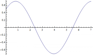
I concluded in my preliminary data post that the ‘Convolve’ function has its limitations and will not work properly with complicated functions. That may be so with relatively obscure functions, but I was wrong in my example. When I computed the convolution the long way by taking the Fourier transform of the product of Fourier transforms, I used the ‘FourierTransform’ function. I should have used the ‘InverseFourierTransform’ function instead. A Fourier transform of a Fourier transform is not necessarily the same as the inverse Fourier transform of a Fourier transform.

If , then through both methods I yield this plot:

Mathematica file: https://vspace.vassar.edu/zerogoszinski/Update.nb

Vspace works better on Macs. If you are not using a Mac, please open the file from the Google Drive folder located at the end of this post. The file name is called ‘Update’.

Deconvolution:

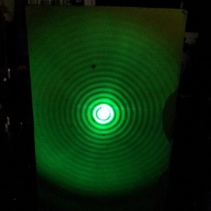
Convolution has applications in imaging, in that a blurry image is simply the convolution of the image and a lens or instrumental function. This function is also called ‘point-spread function’ (PSF). Convoluting two functions is simple since the individual functions are known. Deconvolution is the reverse process, in which you have a convolution and you want to extract the desired image. This requires an understanding of the blurring function, which requires understanding the system that is causing the distortion. Extracting the pure image is much more difficult since every blurring variable needs to be taken into account. A perfect PSF is impossible to determine, so accounting for this function requires good approximations (4). Deconvolution is very important in astronomy, since all data comes from optical based systems. Even a perfect lens convolutes images, as they have unique diffraction patterns. The best focused spot for a camera lens is called the Airy disk:

f is the focal length, is the wavelength, and d is the diameter of the lens.

http://upload.wikimedia.org/wikipedia/commons/thumb/4/4b/Airy_disk_created_by_laser_beam_through_pinhole.jpg/480px-Airy_disk_created_by_laser_beam_through_pinhole.jpg

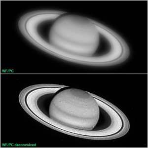
Here is an example of deconvolution in action:

“Experience with the Hubble Space Telescope: 20 years of an archetype”
http://opticalengineering.spiedigitallibrary.org/article.aspx?articleid=1183218

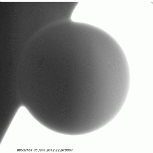
A particularly cool example of the effects of PSF in astronomy is the black-drop effect during the transit of Venus. The black-drop effect is an optical effect where the planet seems to stick to the edges of the star during ingress and pull apart like taffy as it enters the surface. Calculating the transit time would determine the orbital period of Venus. Kepler’s third law would then determine the radius of orbit. Astronomers of the 18th and 19th century wanted to figure this out in order to determine the actual size of the solar system. The black drop effect made it difficult to determine the exact moment Venus entered the Sun’s surface. The cause for this effect was discovered to be mostly due to PSF (Schneider, G., Pasachoff, J. M., Golub, L., 2004, Icarus, 168, 249). Poor optics creates this optical illusion, and accounting for point-spread function [and solar limb darkening] eliminates this effect.

Click to see the animation.
Created by Zeeve Rogoszinski using data taken from Big Bear Solar Observatory.
http://imgur.com/p19moKI

As you can see convolution and deconvolution have important applications in optics. Light beams get distorted as they pass through matter, and the scientist needs to be able to determine what exactly he or she is looking at. If I had the time I would have tried to deconvolute my convolution in the previous post, and try to extract one of the optical filters. I would have first assumed I knew what the second filter looked like, and try to work out the procedure from there. I would then assume I have no idea how the filters behave, and try to blindly deconvolute the filters. This would require looking into the theory behind deconvolution in a more rigorous manner.

Transit Paper:

http://web.williams.edu/Astronomy/eclipse/transits/Schneider_jmp_lg_Icarus2004.pdf

All of my data:

https://drive.google.com/folderview?id=0BxRRP3LUVuftVmFCcnNPMWFhU1k&usp=sharing