Category Archives: Fall 2016

Computational Physics Projects Fall 2016

Fourier Analysis of Unemployment Rate in U.S.

Overview:

Throughout the course in computational physics this semester, I learned how to apply Matlab to different concepts and lessons in physics. I wanted to apply what I learned and collaborate them with ideas and materials from my major in Economics. For this project, I analyzed the data of the unemployment rate in U.S. using Fourier analysis. The Fourier transform decomposes a function of time into the frequency components that make up the original function. As a result, one can look at the different cycles and waves that make up the function. I look at the percent changes in the unemployment rate monthly from February 1948 to October 2016. The Fourier transform data has the amplitude graphed against its frequency, so I can look at the different cycles of the unemployment rate. The second part of the project was to apply a filter to the Fourier transformation. By applying the low-pass filter, I filter out the high frequency data. Then, I inverse Fourier transform the low-pass filtered data to compare it to the original data. I expected the data to have less noise, because the high frequency data that affect the volatility of the data in low periods will be filtered.

Fourier Transformation:

The first part of the project was to Fourier transform the unemployment data. I needed reliable data recorded frequently, so I used the unemployment rate recorded monthly from the U.S. Bureau of Labor Statistics. Then I had to apply the Fourier transformation.

fo

Eq. 1

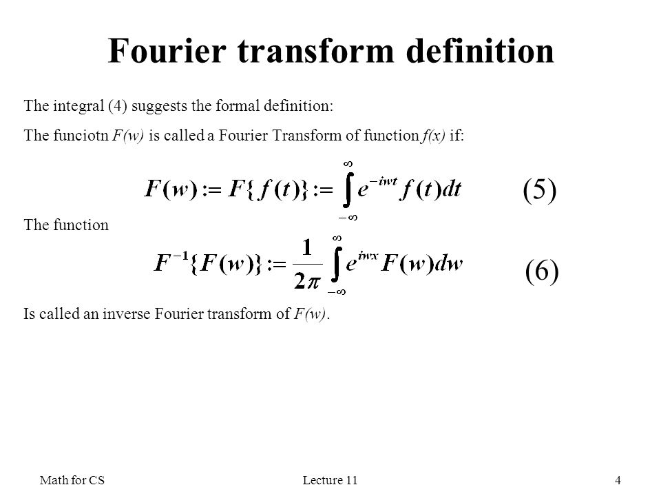
According to Fourier’s theorem, every function can be written in terms of a sum of sines and cosines to arbitrary precision; given function f(t), the Fourier transform F(f(t)) is obtained by taking the integral of f(t)’s sines and cosines function. The exponent factor is just the sum [cos(2*pi*frequency*t)-i*sin(2*pi*frequency*t)]. Discrete Fourier transform can be expressed into the next set of equations from the previous ones.

fouriereq

Eq. 2

The top equation in Eq. 2 is the discrete Fourier transform. The bottom equation is used to get the inverse of the Fourier transform or the original function from the Fourier transform equation. Since the equations in Eq. 2 are just a sum of exponential terms, it appears to be a very straightforward numerical evaluation. In reality, discrete Fourier transforms take a very long time to compute. Each term involves computing the exponential factor, which then have to be multiplied by xn and added to the running total. The total number of operations is of order N^2, because each sum for a given frequency component has N terms and there are N frequency components. However, one can see that the exponential terms in the discrete Fourier transform are multiples of one another. This makes it possible to group up terms in the sums in a way you can store those values and reuse them in evaluating the different components of the discrete Fourier transformation. This is how the fast Fourier transformation came about.

With discrete data set of N ~ 1000, I can perform the fast Fourier transform or the FFT to efficiently compute the discrete Fourier transform. Then, I squared the absolute values of the transformed data. Making this change to the data does not affect the data under Parseval’s Theorem that states, “the squared magnitude of the Fourier Series coefficients indicates power at corresponding frequencies.” The reason behind the squaring manipulation was to change the complex numbers to real components for graphing. Then, I graphed the amplitudes that I get from fft against the frequency. The highest frequency was the data being recorded every month, so I had to set the maximum frequency at .5. Bi-monthly data is the lowest period I can get accurate data from due to Nyquist frequency, which states that minimum rate at which a signal can be sampled without introducing errors is twice the highest frequency present in the signal. Any amplitude that belongs to higher frequencies than .5 would have errors. Many Fourier analysis of signals in physics is shown in varying range of Hertz. However, the periods in economic data have relatively very high periods compared to physics data periods measured in degrees of seconds. As a result, the frequency is relatively low in this graph. Also, the frequency is measured in number of unemployment cycles per month.
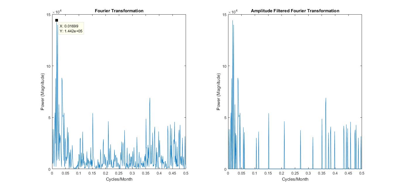
fouriertransform

Figure 1.1

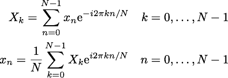
Left side of figure 1.1 shows the graph of the Fourier transformation. The right side just has amplitudes of less than 30,000 amplitude filtered out, so that it would be easier to look at the frequencies with higher amplitudes. One of the challenges of the project was getting the most accurate graph that I can. There are so many different ways the economic data can come out, however, the most accurate graph would have to show evidence that align with known theories in economics.

Analysis:

The frequencies with the highest peaks are the most significant components of the original data. The Fourier transformation graph of figure 1.1 has large peaks near the frequencies of .01699 cycles/month and .3653 cycles/month. These frequencies correspond to 58.858 months/cycle and 2.737 months/cycle respectively.

Business cycles, which include unemployment cycles, are supported very strongly to have cycle length of 5 years on average, which is 60 months. The high peaks that happen above and below the frequency of .01699 are the cycle components of fluctuations that happen in the business cycle. The Cycles do have an average period length of 58.858 months, but cycles can also happen in shorter or longer lengths. The other significant peak range is at 2.737 months/cycle. This aligns with the seasonal unemployment rate; the unemployment rate has a cycle for every fiscal quarter, which is about 3 months. Through these evidences, I can say that the unemployment rate data has been accurately Fourier transformed.

http___www-nber-org_cycles_cyclesmain-1

Figure 1.2

The known theories support the numbers I have, but I also wanted to compare my numbers to the actual numbers. Figure 1.2 is a record of U.S. business cycle expansions and contractions from the National Bureau of Economic Research. They also provide the average cycle (duration in months) of business cycles for both trough from previous trough and peak from previous peak. I looked at peak from previous peak, since the difference wasn’t significant. The average duration of business cycles from economic data of 1859-2009 was 56.4 months, which is very close to the value I got. However, the data also had recorded the average business cycles from 1945-2009. This applies more directly to my transformed data, because my data was from 1948-2016. The average for this period was 68.5 months. I wanted to look at why this data’s average was a bit off from my most significant peak.

The average does fit in the range of the cycle fluctuations, but I figured out that the most plausible reason is that because my transformed data was not smoothed out. One can see in Figure 1.1 Fourier Transformation graph that the business cycle frequency peaks at x=.01699 cycles/month (58.858 months/cycle) and drops to the next point where x=.01335 cycles/month (74.906 months/cycle). The average of the two months/cycle points is 66.882 months/cycle, which is much closer to the data presented in Figure 1.2. If my transformed data were to be smoother with more data points, then the average would have been more accurate.

Low-Pass Filter:

fourierfilteredfinal

Figure 1.3

For the second part of the project, I wanted to apply a simple filter on the transformed data and see how the original data would be affected by that. The idea behind it was to filter out high frequencies above a certain point so that only the low frequency components would be left over for the data. If I were to build up the unemployment function again using the filtered components, what would the original data look like?

I expected the unemployment data to have less noise after the filter, because only the longer period cycles would build up the unemployment rates. I used the inverse Fourier transform function ifft to return the Fourier transformed data back to unemployment rate vs. time graph. The graph on the very right in figure 1.3 is the original unemployment rate graph taken from U.S. Bureau of Labor Statistics. I simply used ifft on the transformed data to return it.

The first step to filtering was to filter the power component of the transformed data, shown in the left, 1st graph of figure 1.3. This wasn’t an accurate representation, because the y axis has been affected by Parseval’s theorem. In order to fix this problem, I filtered the data only applied with fft. The most accurate filter graph I got was the middle graph in figure 1.3.

Analysis:

I made components from 300 to 412 (higher frequency components) equal to 0, so that we would still keep the information about those components and not lose resolution. Then, I inverse Fourier transformed that data. Consequently due to the change of the total length with data, the inverse produces transformed data with different unemployment rates from the original graph, including complex numbers. I was able to only plot the real number components. However, the filter helped me see the general trend of the unemployment rate changes at the exchange of some loss of information; the real number components that I do care about in the middle graph of figure 1.3 represents a more accurate graph of unemployment data with less high frequency noise. The evidence is shown in the decrease in fluctuations of the unemployment rate changes when the middle and right graph are compared in figure 1.3. The rates’ general trend converge more along 0. We do see a time (phase) shifting, but this does not impact the Fourier series magnitude and the inverse.

Conclusions:

The numbers I have gotten through the Fourier Transformation looks accurate and they align with the actual data published. I view my attempt at learning the material and applying it to have been successful. Since, I have used the data from 1948-2016, I should focus on the business cycle published between 1945 and 2009 in figure 1.2. The average of the business cycle is longer post 1945. Assuming that the trend will continue, I can look at the lower frequency end of the most significant peak fluctuation in the Fourier transform graph of figure 1.1. The reasonably lowest amplitude value of the fluctuation range has an x value of .009709 cycles/month, which is about 103 months or 8.6 years.

Our economy has been expanding since the end of the last business cycle, 2009, after the 2008 recession. The decrease in unemployment rate since 2009 has been polynomially decreasing, which indicates we are entering the contraction stage of the business cycle. Since we 7.5 years out of the 8.6 year business cycle I predict has passed, using my data, I can predict that the recession and increase in unemployment rate will happen in the next 1 or 2 years.

Additionally, it would have been interesting to develop filtering methods and programs further so I can get more smooth and accurate data on low frequency business cycles. However, given the time, I believe that the simple low-pass filter was sufficient to show how a filter affects the Fourier transform data and its inverse.

Reference:

NBER. “US Business Cycle Expansions and Contractions.” The National Bureau of Economic Research. NBER, 20 Sept. 2010. Web. 09 Dec. 2016.

Series, Nber Working Paper. Matthew D. Shapiro (n.d.): n. pag. NBER. NBER, 1988. Web. 9 Dec. 2016.

US. Bureau of Labor Statistics, Unemployment Level [UNEMPLOY], retrieved from FRED, Federal Reserve Bank of St. Louis; https://fred.stlouisfed.org/series/UNEMPLOY, November 29, 2016.

MIT. “The Fourier Series and Fourier Transform.” Circuit Analysis (n.d.): 102-23. MIT. MIT, Spring 2007. Web. 9 Dec. 2016.

James, J. F. A Student’s Guide to Fourier Transforms: With Applications in Physics and Engineering. Cambridge: Cambridge UP, 2011. Print.

Share

Numerical Solution to Schrodinger Equation in a 1D Periodic Potential

Summary:

The following article serves as a discussion of a program that I designed to serve as an educational tool for students of introductory solid state physics.  This program calculates the dispersion relation for a particle in periodic 1D potential and presents related information, such as band gap energies and movies of the time-evolved stationary states directly above and below the first band gap.  I begin by introducing the reader to the underlying physical concepts, such as energy gaps, dispersion curves, Bloch’s theorem, and the nearly-free electron model.  I then proceed with a discussion of the program and how it can be used to demonstrate a wide array of phenomena related to to these theoretical topics.  I conclude with a description of how the program operates, its limitations, and suggestions for how this work can be extended in the future.

Introduction:

In many solids, such as crystals and semiconductors, atoms are arranged in an organized and periodic manner. This periodicity in the organization of the atoms leads to an electric potential that is also periodic in space. Describing the behavior of particles, such as electrons, in such potentials is a primary topic in any introductory solid state physics course, and remains an important area of research in modern electronics.

An interesting phenomenon that occurs in periodic potentials, and a topic which is at the heart semiconductor device operation, is the presence of energy bands. In many solids, there are intervals of allowed energies which particles experiencing that potential can take. That is, if one were to measure the energy of an electron in a periodic potential, they might measure values anywhere between two energies, say, a and b, but nowhere between two other energies, say c and d. The allowed energy intervals are known as energy bands and the energy difference between two bands is known as a band gap [1].

In introductory solid state texts, such as “Solid State Physics,” by Kittel, the origin of the band gap is often presented in the context of the nearly-free electron model [1]. In the nearly-free electron model, electrons are described as free particles with an effective mass that depends on the electron’s wavenumber. The energy gap is then explained conceptually as being due to the existence of standing waves that form when the wavelength of the electron is some harmonic of the periodicity of the potential. Two distinct standing waves form, one in which the electron’s wavefunction is concentrated around regions of high potential energy, and one in which the electon’s wavefunction is concentrated around regions of low potential energy. The energy difference between these two standing wave states is taken as the bang gap energy.

While presenting band gaps in this way avoids grappling with the full complexity of quantum mechanics, band gaps are an essentially quantum mechanical phenomenon. By the time many students begin studying solid-state physics, they have already studied at least one of the archetypal quantum mechanics examples, such as the infinite square well or the hydrogen atom. Furthermore, they have learned that only certain energies have associated normalizable solutions to the Schrodinger equation, and that these are the measurable energies of the system. The only difference in infinite periodic potentials, is that instead of discrete energy levels, there are intervals of allowed energies. The goal of this project is to help students bridge the gap between the conceptual nearly-free electron model and the results of quantum mechanics.

Bloch’s Theorem:

One of the most important theorems involving solutions to the Schrodinger equation in a periodic potential is Bloch’s theorem. This states that the normalizable solutions to the time independent Schrodinger equation in a periodic potential have the form \psi_k=u_k(\vec {r})e^{i \vec{k} \cdot \vec{r}}, where \vec{r} is the position vector, \vec{k} is the wave vector, u_k(\vec {r})=u_k(\vec {r}+\vec{T}), and \vec{T} is a lattice vector (the position vector between two lattice sites) [1]. In one dimension, this reduces to the criterion that \psi_k=u_k(x)e^{ikx}, where u_k(x)=u_k(x+na), a is the periodicity of the potential, and n is an integer. It follows from Bloch’s theorem that if \psi_k is a solution to the Schrodinger equation, then \psi_{k+G} is also a solution, provided that G=\frac{m \pi}{a} for some integer m [1]. It is common to plot the allowed energies against k for \frac{- \pi}{a} < k < \frac{\pi}{a} (known as the first Brillouin zone), as this gives a complete account of the allowed energies of the system [1]. The energy of the allowed wavefunctions as a function of k is known as the dispersion relation or dispersion curve [1].

Project and Results:

I created a program that calculates the dispersion relation for three 1-dimensional periodic potentials, a square, triangle, and sinusoidal wave (figure 1).

Fig 1: Periodic potentials which are available which are available to be solved by simulation. This is understood to represent a single cell of the potential functions. The true potentials infinitely many cells sewn together at the edges.

Fig. 1: Periodic potentials available available in the program. This is understood to represent a single cell of the potential functions. The true potentials repeat infinitely many times in both the positive and negative spacial directions.

This program is intended as an educational tool for students of solid-state physics who are beginning to study the concept of bang gaps. It calculates the dispersion curves by finding the first several allowed energy eigenstates (of the potential of interest) for a discrete selection of k values in the first Brillouin zone. It then plots the energies of these states against the wave number, k, which gives the dispersion curve (figure 2). The first several band gaps are evident as the empty regions between dispersion curves.

tr

tr1

Fig. 2: Dispersion relations calculated by the program. The top image corresponds to the triangle-wave potential, the middle image corresponds to the sinusoidal potential, and the bottom image corresponds to the square-wave potential. Regions between the colored horizontal lines represent band gaps.

The program also produces a movie of the time-evolved eigenstates on either side of the first band gap (figures 3 and 4). In these movies, it is worth noting that the state just above the first energy band is concentrated around high-energy regions of the potential and the state just below the first band is grouped around low-energy regions of the potential. One can also see that the periodicity of the allowed wavefunctions on either side of the gap is indeed a harmonic of the periodicity of the potential (actually a sub-harmonic). These results demonstrate that the qualitative explanation of band gaps provided by the nearly-free electron model is in close agreement with the results of quantum mechanics.

www-gifcreator-me_jyqlj

Fig. 3: Animation of the real and imaginary parts of the wavefunction just below the first band gap (click image to see animation)

Fig. 4: Animation of the real and imaginary parts of the wavefunction just above the first band gap (click image to see animation)

Along with having several types of potentials to choose from, the height and periodicity of the potential are left as variable inputs for students to change and explore. By changing these values, students can begin to build and intuition for how the structure of the dispersion curves depend on the size and shape of the potential. For instance, by decreasing the height of a potential of fixed periodicity, students are able to watch the structure transition from being an insulator (large band gap), to a semiconductor (small band gap), to a metal (little or no band gap) [1].

Fig. 4 Dispersion relation for decreasing magnitude of the potential barriers. The decrease in energy gaps between dispersion curves represent the transition from insulator to conductor.

Fig. 5: Dispersion relations for decreasing magnitude of the potential barriers. The decrease in energy gaps between dispersion curves demonstrate the transition from insulator to conductor.

The program can also be used as a tool for students to build a better understanding of Bloch’s theorem. For instance, by instructing the program to calculate the allowed energies for values of k beyond the first Brillouin zone, we see that the dispersion relation is periodic in k (figure 6). This corresponds to the result from Bloch’s theorem that if \psi_k is a solution to the Schrodinger equation in a periodic potential, then \psi_{k+G} is also a solution [1].

Fig. 5 Dispersion relation, which is periodic in k

Fig. 6: Representative dispersion relation that extends beyond the first Brillouin zone.  Note the periodicity in k, as predicted by Bloch’s theorem.

Verification of Results –  The Kronnig-Penney Model:

In order to demonstrate that this program produces solutions that are in agreement with theory, I considered the square-wave potential. This potential corresponds to the Kronnig-Penney model, which has been studied extensively. There is an analytic solution for the allowed energies of this potential in the form of roots to a transcendental equation [1]. Much like the methods employed by this program, this expression is found using Bloch’s theorem to determine appropriate wavefunction boundary conditions.

This equation for the allowed energies has been used to find the analytic dispersion curve for the Kronnig-Penney model. This is plotted along with the dispersion curve determined by the numerical methods employed in this program (figure 7). Indeed, the two dispersion relations are in excellent agreement, which demonstrates that this program does reliably calculate the allowed energies for a 1D periodic potential.

Figure 1: The top image shows the dispersion curve for the square-wave potential calculated by numerical methods. The bottom image shows the dispersion curve calculated using analytic results obtained from Bloch's theorem.

Fig. 7: The top image shows the dispersion curve for a square-wave potential calculated by numerical methods. The bottom image shows the dispersion curve calculated using analytic results obtained from Bloch’s theorem.

A more in depth discussion of the Kronnig-Penney model can be found in “Solid State Physics,” by Kittel [1].

Program Operation:

In order to determine the allowed energies of a particle in a periodic potential, I employed the numerical methods discussed in “Numerical Solution of the 1D Schrodinger Equation: Bloch Wavefunctions,” by Dr. Constantino Diaz [2]. The theory and operation of the procedure outlined in this paper is structured in the following way. The time independent Schrodinger equation is a second order differential equation in x, so there exists two linearly independent solutions for each value of E, which we will denote as \psi_C(k,E,x) and \psi_S(k,E,x) [2,3]. In other words, any wavefunction with wavenumber k and energy E, is expressible as a linear combination of \psi_C(k,E,x) and \psi_S(k,E,x). That is, \psi_k(E,x)=A\psi_C(k,E,x)+B\psi_S(k,E,x) for some complex numbers A and B [2,3].

\psi_C(k,E,x) and  \psi_S(k,E,x) are determined for a chosen value of k by using the Schrodinger equation to calculate the wavefunction in discrete steps [2]. This is done by expressing the Schrodinger equation in finite difference form:

    \[\frac{\hbar^2}{2m} \frac{d^2}{dx^2} \psi+V\psi=E\psi \approx \frac{\hbar^2}{2m} \frac{\psi_{n+1}+\psi_{n-1}-2\psi_{n}}{\Delta x^2}+V_n \psi_n=E\si_n,\]

where V(x) is the potential function, m is the particle mass, \Delta x is the spacial step size, and n denotes the n^{th} spacial spacial step [3]. Rearranging terms gives:

    \[ \psi_{n+1}=\frac{2m(\Delta x^2)}{\hbar^2}(E-V_n)\psi_n-\psi_{n-1}+2\psi_n,\]

which can be used to calculate the wavefunction for some guess value of E [3].  Since the potential functions are symmetric, initial conditions of \psi_C(\frac{a}{2})=1, \frac{d\psi_C}{dx}(\frac{a}{2})=0 and \psi_S(\frac{a}{2})=0, \frac{d\psi_S}{dx}(\frac{a}{2})=1 can be chosen without loss of generality [2,3].

According to Bloch’s theorem, \psi(a)= u_k(a)e^{ika}=u_k(0)e^{ika}=\psi(0)e^{ika}, and \psi^{'}(a)= u_k^{'}(a)e^{ika}+iku_k(a)e^{ika}=u_k^{'}(0)e^{ika}+iku_k(0)e^{ika}=\psi^{'}(0)e^{ika} [1,2]. These boundary conditions can be expressed in terms of the coefficients A and B as A\Delta C+B\Delta S=0 and A\Delta C^{'}+B\Delta S^{'}=0, where \Delta C=\psi_C(a)e^{\frac{ika}{2}} -\psi_C(0)e^{\frac{-ika}{2}, \Delta S=\psi_S(a)e^{\frac{ika}{2}} -\psi_S(0)e^{\frac{-ika}{2}, \Delta C^{'}=\psi_C^{'}(a)e^{\frac{ika}{2}} -\psi_C^{'}(0)e^{\frac{-ika}{2}, and \Delta S^{'}=\psi_S^{'}(a)e^{\frac{ika}{2}} -\psi_S^{'}(0)e^{\frac{-ika}{2} [2]. For this system of equations to be satisfied, the determinant of the coefficients must be equal to zero. That is, the allowed energies for a given value of k satisfy the equation, G(E)=\Delta C \Delta S^{'} - \Delta S \Delta C^{'} =0. If G(E)=0, then E is taken as an allowed energy [2]. If not, then a new value E+\Delta E is treated as the energy and new values of \Delta C, \Delta S, \Delta C^{'}, and \Delta S^{'} are computed. This process is repeated many times so that several allowed energies are found for the chosen value of k. The whole procedure is then repeated for evenly spaced values of k in the first Brillouin zone.

Program Limitations:

The primary limitation of this program is its sensitivity to choices of step size.  If \Delta E is chosen to be too small, an insufficient number of roots are found for G(E) to create a viable dispersion curve.  If the energy step size is chosen too large, then the program is unable to locate the zeros of G(E), particularly at the ends of the first Brillouin zone.  In both of these instances, the program stops running and produces plot of G(E) for the last calculated value of k. If this graph has less than four roots, then the step size was chosen to be too small.  If the graph has many roots, but the program still failed, then the step size was chosen to be too big. The program seems to be most effective if \Delta E is chosen to be roughly one percent of the maximum of the potential functions.

The program also fails to produce reliable results if the spacial step size is chosen to be too large.  As long as the spacial step size is no more than five percent of the width of the potential barrier and 0.5 percent of the periodicity of the potential, the program seems to operate normally.  The program also produces poor results if the step size in k is chosen to be too large, but this only decreases the resolution of the dispersion curve.  An overly large choice in the step size of k will not result in a failure of the program unless it is chosen to be comparable to the size of the first Brillouin zone. As long as operators are aware of these problems, the program performs well.  Still, I recommend that only small changes in the parameters of the potential be made each time the program is run so that the user is able to adjust the step sizes gradually.

Future Work:

A good continuation of this project would be to alter the program to accommodate for potentials that are not symmetric about the point x=\frac{a}{2}
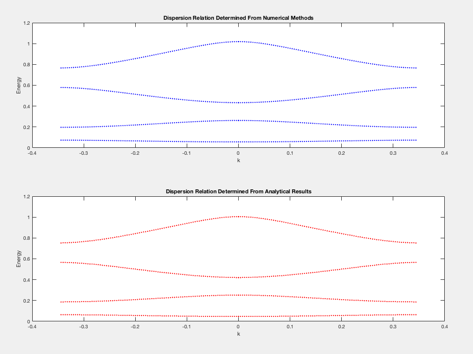
. Suggestions on how to implement this modification can be found in “Numerical Solution of the 1D Schrodinger Equation: Bloch Wavefunctions,” by Dr. Constantino Diaz [2]. An even more interesting progression of this work would be to write a program that can solve the Schrodinger equation in a two or three-dimensional potential lattice. The particular method employed in this program is not generalizable to higher dimensions, but other methods that also apply Bloch’s theorem to provide appropriate boundary conditions can be applied to periodic potentials of higher dimension [2]. In the case of higher dimensional potentials, the dispersion relation is anisotropic with respect to spatial orientation. Qualitatively, this is due to the fact that the spacing between potential barriers is different along distinct spatial directions [1]. A program that could allow students to explore this directional dependence of the dispersion relation and plot the associated wavefunctions could be a helpful tool to solidify the effect of spatial anisotropy on wavefunctions in crystals.

Conclusions:

I created a program that calculates the dispersion relation for a particle in a 1D periodic potential, which can be used as a educational tool for students of solid state physics.  It uses the discrete version of the Schrodinger equation along with boundary conditions provided by Bloch’s theorem in order to find the first several allowed energies for values of k in the first Brillouin zone.  Comparison of the results of this program to the analytic solution for the dispersion relation of Kronnig-Penney demonstrates that this program provides valid results. The program demonstrates several key properties of wavefunctions in a periodic potential, including energy bands, the distribution of wavefunctions on either side of the band gap around high and low regions of the potential function, the dependency of energy gaps on the height of potential function, and the periodicity of the dispersion curve predicted by Bloch’s theorem. A good continuation of this work would be to incorporate non-symmetric potential functions or to construct a procedure for calculating the dispersion relation in higher dimensional potentials.

References:

[1] Kittel, Charles. Solid State Physics. 8th ed. New Caledonia: John Wiley & Sons, 2005. Print.

[2] Uteras Diaz, Constantino A. “Numerical Solution of the 1D Schrodinger Equation: Bloch Wavefunctions.” Numerical Solution of the 1D Schrodinger Equation: Bloch Wavefunctions. ARXIV, 23 Mar. 2005. Web. 10 Dec. 2016. <http://cds.cern.ch/record/828907/files/0503171.pdf>.

[3] Giordano, Nicholas J. Computational Physics. 2nd ed. Upper Saddle River, NJ: Prentice Hall, 2006. Print.


Share

Orbital Motion of Our Solar System

Overview:

For my final project, I made two animations that model the orbital motion of planets in our solar system based on data sets that I generated. The first animation shows the orbit of the inner planets and the second shows the full solar system. While the spacing of the planets is to scale, the size of the planets is not. The sun and eight planets are simulated in two-dimensional plots with the sun at the origin (sorry Pluto!). The plots are in the reference frame of the sun, so the sun is at rest. The planets are color-coded based on the dominant color of their surface (i.e. yellow for the sun, red for Mars, etc). The full orbital paths are shown in the plots along with the moving planets for reference. The plots show at least one full revolution for each planet. This program was created for educational purposes. My intentions are that this program could be shown to children learning about the solar system to give them an idea of the scale of the solar system relative to Earth and a visual representation of the difference in orbital periods.

Background, Methods, and Assumptions:

The data sets were generated using the Euler-Cromer method. I made several key simplifying assumptions that led to the model I used. I assumed that the sun is exactly centered in each planet’s orbit. I assumed that the effects of gravity were only between an individual planet and the sun, with planets having no effect on each other. By also assuming the orbits are circular, we equate the centripetal force to the force of gravity to get a zero net force. Using units of AU, we get that the gravitational constant G, multiplied by the mass of the sun, Ms, is equal to 4π2. Solving the equation then gives us the following equations to calculate the x and y components of the position and velocity for a planet of mass M:

screen-shot-2016-12-09-at-10-21-53-pm

As both the centripetal force equation and gravity force equation have the planet’s mass involved, the final equations surprisingly do not end up involving a factor of the mass. The use of the Euler-Cromer method comes in to play for the position equations, where the velocity calculated for time i+1 is used instead of the velocity from time i (the previous time, as would be used in the Euler method).  I initialized the positions of the planets to be at their respective average distance from the sun along the x-axis. The initial velocity at this point of the orbit is completely in the y-direction. It was calculated by dividing the circumference (still assuming a circular orbit) by the period in terms of an Earth year (for Earth, the initial velocity was 2π AU/Earth year). Based on these initial conditions, I looped through the equations over a time window of 300 with a time step of .005 to generate my data. This process was repeated for each planet using essentially the same code but with different initial positions and velocities. Once I had my data calculated, all that was left was to plot. The orbits calculated are not consistent as the planets make successive revolutions about the sun, resulting in an overlapping ellipse pattern when the full data set was plotted. I plotted a section of the data for each planet that included one orbit to show the path. The for loops plotted one position pair at a time successively, resulting in the animated planets orbiting the stationary sun.

Visualizations:

innerplanetsInner Planets Simulation

solarsystem Full Solar System Simulation


Results

As I was trying to model an existing system, I had information to compare my results with. The main way I judged the effectiveness of the program is the relative orbital periods of the planets. The real orbital periods compared to Earth are shown in the following table:

Planet Approximate Earth orbits per one orbit
Mercury .24
Venus .62
Earth 1
Mars 1.9
Jupiter 11.9
Saturn 29.4
Uranus 83.7
Neptune 163.7

For one Earth period, Mercury should undergo about four and an eighth periods and Venus should have one and two-thirds periods. Using somewhat qualitative observations by tracking the planets in the animations, I found that my program has very accurate relative orbits as compared to the exact data. My orbits are, however, seem more elliptical than they should be.


Discussion:

A number of the simplifying assumptions made are blatantly not correct. The assumption made that the orbits are circular is not true, especially for Mercury, which has a higher eccentricity. I found it quite interesting that, despite creating the model around circular orbits, the calculated orbits ended up being elliptical. Assuming that the sun is centered in the orbits is wrong, as Kepler’s laws state the sun should be at one focus of the orbit. As the orbits are not actually circular, this means that the sun would not be centered (although most planets have a low eccentricity so this would be only a small shift). The time step used must be quite small, or else the orbits will break down (this happens very quickly for Mercury as the time step is increased). I made the decision to have two animations in order for the inner planet orbits to be clearly observable. In the full solar system plot, it is clear that the periods of the smaller planets run much shorter than the outer planets. Apart from that fact, little else can be seen regarding those orbits due to the scale of Neptune’s distance from the sun. The length of Neptune’s period compared to the rest of the planets created other issues as well. The animations themselves take a long time to run, which is somewhat necessary to have a complete cycle for Neptune.  Another limitation is the amount of computation used in the animations. I ended up using 32 vectors with 60000 entries each to hold all the data, along with several other variables to hold enough information to track a full revolution for Neptune. The visualizations lack legends when the code is run. When legends are included in the plots, the time between frames in the animation was reset from what I coded it to be and the animation slowed down substantially. For this reason the code for legends was commented out in the Matlab program (it can be uncommented if legends are desired at the user’s risk of very long runtimes for the animations). For the visualizations, I was able to override the time in between images in the .gif, and so legends are included in the figures shown.


Conclusion:

I was able to successfully and accurately model a somewhat simplified version of our solar system. The Euler-Cromer method was appropriate for this task and I would continue to use it in further investigations. In terms of moving forward with this program, my next steps might be making the program interactive. This process would include allowing the user to select the number of planets, the mass, radii, color, and other parameters. It would also be nice to incorporate moons into the simulation. In terms of improving the current program, I would try to figure out a way to include the legends in the program without disrupting the speed of the animations in the code (this would especially be necessary if the program was interactive). Creating an algorithm to optimize the number of data points needed to have one full period for each planet would also be useful to streamline the data.


References:

Giordano, Nicholas J., and Hisao Nakanishi. Computational Physics. 2nd ed. Upper Saddle River, NJ: Prentice Hall, 2006. Print.

“Kepler’s Laws.” HyperPhysics. N.p., n.d. Web. 30 Nov. 2016.

Williams, David R. “Planetary Fact Sheet – U.S. Units.” NASA. NASA, n.d. Web. 20 Nov. 2016.

Share

Modeling a Binary Star System

Overview:

The stated goal of this project was to create a set of simulations to be used in an educational environment to better understand the orbital dynamics of a binary star system by plotting, in 2-D, the x and y positions of the celestial objects within the system. This project was split up into four subsections, or subprograms within the program. The first subprogram considered a simple binary star system, the second a system with stars that had different velocities, the third a system with stars that had low velocities, and the fourth a simple system with a planet orbiting one of the stars. We deviated slightly from our project plan because we were unable to explore the effects of mass on the orbits of the stars; this was because of an issue that arose within our model, prohibiting us from being able to accurately assess the effects of mass. Here, we present our results and conclusion of our project. The method section has been omitted, but can be found within our program for each subprogram.

Results:

All of our subprograms self-generated data, based on some initial parameters, and plotted that data on graphs for N iterations. We have attached our graphs here in the form of clickable GIFs. The number of iterations N is responsible for the accuracy of our orbits. In our programs, we use low values for N to obtain semi-accurate orbital data without expending too much computational power or too much time. This is why our orbits may not seem to completely line up; if we increase N to around a thousand or fifteen hundred, then we will see that the orbits will line up quite well. It is important to note that the dots are representative of the velocities of the celestial objects. If there is a cluster of consecutive dots, that indicates that the celestial objects are moving with constant velocities; however, if consecutive dots are far apart, that indicates that the celestial objects are moving with increasing velocity. Additionally, the units used here are not standard units; our position units are in AU, our velocity units are of the form 2πAU/yr, and our mass units are in kg. Below we discuss the results of each subprogram.

I. Simple Binary Star System:

sbss

Figure 1.1: Results of Program 1. Click on image to see GIF simulation.

For our first subprogram, as mentioned previously, we tried to generate a simple binary star system. Our initial parameters were as follows:

For star 1, x = .72, y = .64, V_x = 2.42π, V_y = 0, and M = 5*10^30.

For star 2, x = -.72, y = -.64, V_x = -2.42π, V_y = 0, and M = 5*10^30.

Note that our masses for our stars here are equal (5*10^30 kg). We compared our results, shown in Figure 1.1, to some simulations online, which also had the stars being of equal mass: 1 and 2. Our simulation seemed to be in line with these results. We can also understand why our result makes sense using our knowledge of physics. First, we must consider the following equation:

bc8ad1167d8a4def851ec3df6394bcccThis is the equation for gravitational force between two celestial objects with masses of M_S and M_E. Since our binary star orbit is supposed to be stable, F=F_G=ma. If the objects are close together, then the gravitational force between them is maximized, but because this has to be equal to ma, acceleration must increase since mass cannot be changed. This increase in acceleration is the reason for the increase in velocity. Similarly, if the objects are far apart, then the gravitational force between them is minimized and we expect acceleration to decrease, so the velocities of the objects will approach a constant value.

II. What if the Stars have Different Velocities?

wsdv

Figure 1.2: Results of Program 2. Click on image to see GIF simulation.

Once we were able to generate the simple binary star system, we wanted to see the effects on the orbits due to a change in velocity. For this program, our initial parameters were:

For star 1, x = .72, y = .64, V_x = 2.6π, V_y = 0, and M = 5*10^30.

For star 2, x = -.72, y = -.64, V_x = -2.42π , V_y = 0, and M = 5*10^30.

We increased the V_x of star 1 to 2.6π and kept star 2’s V_x at -2.42π, the same as in subprogram 1. The results can be seen in Figure 1.2. It is, however, important to note a flaw on our method. Namely, we assigned mass to the common barycenter of the stars. This was initially useful to stabilize the orbits of the stars, but as seen here, it makes it so that the orbit star 2 is not affected by that of star 1. We did, however, expect the orbit of star 1 to be more elliptical with a higher velocity because an increase in velocity would mean that the star would be getting closer to its escape velocity, at which point it would move in a straight line.

III. What if the Stars have Low Velocities?

Figure 1.3: Results of Program 3. Click on image to see GIF simulation.

Figure 1.3: Results of Program 3. Click on image to see GIF simulation.

Next, since we were unable to consider changes in mass, we considered the case where the velocities of both stars were very low. For this program, our initial parameters were:

For star 1, x = .72, y = .64, V_x = 1.5π, V_y = 0, and M = 5*10^30.

For star 2, x = -.72, y = -.64, V_x = -1.5π, V_y = 0, and M = 5*10^30.

Note the decrease in velocity from 2.42π and -2.42π to 1.5π and -1.5π for star 1 and star 2, respectively. The result we obtained is shown in Figure 1.3. This result is rather interesting because it seems that the orbits of the stars are moving in a counterclockwise direction through space. However, this orbit is not stable because, after some time, the stars would both escape the system (we know this because we ran this for many iterations before, but did not display it here). We attempted to find a simulation online for comparison, but we were unsuccessful in doing so. However, given that this is built on the program of the simple binary star system, which we know is fairly accurate, we can assume that this may also be a fairly accurate representation.

IV. Simple Binary Star System with a Planet:

Figure 1.4: Results of Program 4. Click on image to see GIF simulation.

Figure 1.4: Results of Program 4. Click on image to see GIF simulation.

This subprogram is the one that we built up to using our previous problems. With a good grasp of the flaws of our system and the orbital dynamics of a simple binary star system, we introduced a planet. Below are our initial parameters:

For star 1, x = .72, y = .64, V_x = 2.42π, V_y = 0, and M = 5*10^30.

For star 1’s planet, x = .3, y = .3, V_x = .09π, V_y = 0, and M = 2*10^24.

For star 2, x = -.72, y = -.64, V_x = -2.42π, V_y = 0, and M = 5*10^30.

The result of our program can be seen in Figure 1.4. It is important to note the initial behavior of the planet. Initially, the planet is assisted by the gravitational force of its host star (since their initial velocities are in the same direction) and moves very quickly outside of the system, but because of the gravitational force of its host star, it is then pulled into an orbit around it. The behavior of the planet is interesting because, as its host star moves, it attempts to stay in orbit by moving along with it. This was to be expected. However, after some time, the planet exits the system. This indicates that this orbit is highly unstable. Although, much time was spent attempting to find a stable orbit with no success. This could explain why we were also unable to find a simulation for comparison – it seems extremely rare or difficult for a planet to be in a stable orbit in a binary star system. Although it must be noted that we had only taken into account the gravitational force on the planet by its host star; previously, we experienced crashes of MATLAB when we attempted to consider the gravitational force of both stars on the planet.

Conclusion:

Referring to our project plans, we were able to achieve most of what we aimed to do. We also believe that this set of simulations can be useful in an educational environment for students. However, because of our model, the only thing we were not able to accurately assess was the effect of mass on a binary star system. Although there are already some interactive simulations online, such as this one, that do so. We experienced a lot of difficulty in building our initial model because we were attempting to replicate an example outlined in Computational Physics. However, we managed to create a good base program to explore further simulations. If we can continue to build on this model, we may consider working out the kinks with taking into account the gravitational force of star 1 and 2 on star 1’s planet. Additionally, it would be interesting to consider multiple planets in different orbits around this binary star system.

References:

“Binary Star.” Wikipedia. Wikimedia Foundation, n.d. Web. 28 Nov. 2016. <https://en.wikipedia.org/wiki/Binary_star#Center_of_mass_animations>.

Fix, John D. “Interactives.” Interactives. N.p., n.d. Web. 28 Nov. 2016. <http://highered.mheducation.com/sites/0072482621/student_view0/interactives.html#>.

Giordano, Nicholas J., and Hisao Nakanishi. Computational Physics. 2nd ed. Upper Saddle River, NJ: Prentice Hall, 2006. Print.

Zingale, Michael. “Introductory Astronomy Animations (and Figures).” N.p., n.d. Web. <https://zingale.github.io/astro_animations/>.

Share