(Revised 5/7/14)

Initially, I intended to model capacitors of various shapes, including more realistic configurations like rolled-up plates or variable (i.e. adjustable) capacitors. Though these configurations were not ultimately simulated, the information gathered, looking only at square parallel plate capacitors, was illuminating, and the foundational programs I wrote could, with some manipulation, be extended to more complicated arrangements.

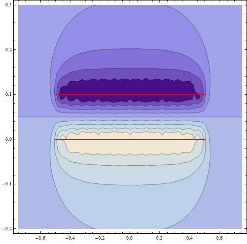
The method I ended up using, detailed extensively in the data post, was relatively efficient but still took a non-trivial amount of time (see below) to simulate the electric fields that dictate the properties of a capacitor. The size of grid I used (averaged over two grids: one with 211^2 = 44521 points, the other with 212^2 = 44944 points) was chosen so that the simulated electric fields were at least 99.9% accurate over the distances examined and so that the simulations took no more than 10 minutes each to run (6 plate simulations were run in total, resulting in an hour of pure computation; note that by taking advantage of plate symmetry, this was actually 1/4 the time one might have expected, as it took about 2.4 seconds to find the E-field at any point).

Accuracy of the method at calculating the E-field was checked at a few points against the computationally inefficient but presumably 100% accurate theoretical model, which is based on fundamental physics (integral Coulomb’s law). This method took up to 10 minutes to calculate the E-field at an arbitrary point near the capacitor, though it was much faster far away from the capacitor (where we are naturally not interested).

Splitting a shape into thousands of manageable quantized points charges (each producing a field in accordance with Coulomb’s law for point charges) proved to be an effective tool, even for the relative simple square plates studied here. This method could be expanded in the future to much more complicated surfaces or even volumes to accurately model the electric field of complex shapes that would otherwise be hopeless to analyze analytically. Of course, a real charged object is charged with a finite number of charge carriers, so this method is not physically unsound (on the other hand, a plate charged to 10^-6 C like mine would need 6.25 x 10^12 electrons spread over it rather than a mere 44,000)

It should be noted that I did not examine the effects of dielectrics placed between plates. Though this was originally planned, I omitted doing this not out of time constraints, but rather because it would not have proved particularly illuminating. Linear dielectrics (the only kind extensively analyzed in 341) have very straightforward effects on energy storage and capacitance, which do not seem to depend on capacitor dimensions. Equation 4.58 and an unlabeled equation on page 197 make this clear (Griffiths, 4th ed.):

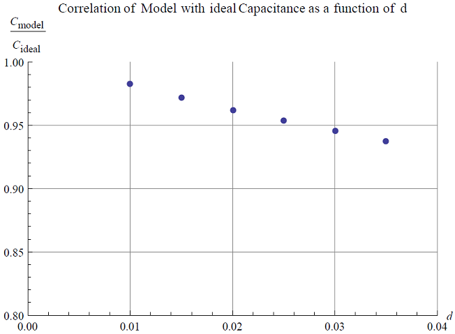
Overall, this project was an excellent exercise in computation and matrix manipulation (the data for the electric field at a set of points above a plate was stored in a 3 by 1024 matrix, for example). It was also very useful for practicing using approximation methods based on fundamental physics to solve an otherwise complicated problem. In the end, the ideal model of a capacitor was shown to be insufficient for extremely accurate capacitor parameters at all but the closets plate separations. Of course, real capacitors have by their design very close plates to maximize capacitance, so the choice of method depends on one’s needs and situation.

Perhaps the most useful “next step” would be to take the data for more plate separations and fit a curve to the points, resulting in a function for capacitance or energy as a function of plate separation. Based on the few points I took (see the animation), such a function is approximately a straight line for very small separations (i.e. the ideal approximation) but diminishes with distance like a square root function.

The code used to run these simulations could be expanded upon to use for visualizing electric or potential fields, or for any other application where an arbitrarily complicated electric field (or possibly a gravitational field) needs to be modeled. I tried to keep a neat, albeit very lengthy, notebook file, though I could have labeled my graphics and the computation times more clearly (I used the Timing function on almost every computation, but the way Mathematica returns the timing value is not extremely conspicuous).

Abstract:

Using an approximation designed for this project, the energy storage capability as well as the capacitance of several simple, slightly physically impractical, square parallel plate capacitors were found. Compared to the idealized model taught in introductory physics, these capacitor store 90% to 97% the energy and have 94% to 98% the capacitance. These discrepancies are caused by the finite dimensions of the plates, which result in fringing effects at the edges. The accuracy of my model is likely high, based on a comparison of the approximations used and a sampling of values produced by the exact, theoretical model, which itself proved too computationally intensive to use extensively  with the resources available. Overall, the discrepancies from the ideal model are fairly significant (a few percentage points) at the plate separations studied, indicating that this method could be quite useful for electronics applications. At closer, possibly more realistic plate separations, this relatively complicated model may prove too time consuming to justify its use over the ideal model, which represents the limit as separation approaches 0.

Methods:

Using Coulomb’s law for one particle , a massive grid of tens of thousands of points charges spread evenly across a predefined area could be constructed. The field of this grid was then compared at a few points to the field of the exact, theoretical values predicted by the more general (but not most general) form of Coulomb’s law:

,

or more explicitly:

This was to determine how accurate the approximation was, though the exact method could not be used all the time as it was determined to be very computationally inefficient.

Plotting the electric field magnitude of a cross-section of the grid configuration like that described above, it is clear that the quantized nature of the grid disappears far away from it, but up close there are sharp irregularities (red lines represent the plates that are being modeled). Fringing effects can also be seen (note that a vector field proved too computationally intensive to plot). The configuration below is for a 14 by 14 grid for computational ease, much less fine that the 211 by 211 grids used in the simulations.

 

 

 

 

 

 

 

The field of a fine grid at thousands of locations within the capacitor was then calculated. From here, all parameters depending on E (the most important of which are energy storage, W, and capacitance, C) could be determined using:

(Griffith’s 4^th Ed. eq. 2.45 and 2.55) where potential difference is V = Ed, an approximation from the ideal model used in the interest of time (though the E used was not the ideal values). Note that d = plate separation. Also note that the first equation was used in summation form  (V here is volume) due to the quantization of the data (i.e. there was no easily integrable function for E).

Raw Data:

This project dealt with very large matrices (several were 3 by 1024) to examine the slightly variable electric field within a capacitor, and as such, much of that data is not of interest. The end results of these computations, however, are. The plates for all capacitors simulated were 4 square meters and had positive or negative 10^-6 Coulombs on them, with separation distance the only parameter being varied. Separation distances used were 0.01 meters, 0.015 meters, 0.02 meters, 0.025 meters, 0.03 meters, and 0.035 meters. Respectively, the energy that these capacitors stored in the space between the plates were (in milli-Joules): 0.137452, 0.202963, 0.266781, 0.328944, 0.38957, and 0.448766. Their respective capacitances were (in nano-Farads, a fairly typical capacitance unit (Griffiths 105)): 3.47951, 2.29386, 1.70372, 1.3506, 1.11583, and 0.948688.

Compared directly to the values predicted by the ideal model (namely that  and , A = area of one plate), the respective energy storage values are 97.36%, 95.84%, 94.49%, 93.20%, 91.98%, and 90.82%, while the respective capacitance values are 98.24%, 97.15%, 96.21%, 95.34%, 94.52%, and 93.75% (capacitance data is seen in the figure below).

So, while the values attained from both models are similar, the ideal model always overestimates the performance of the capacitor. To visualize the effect of plate separation on capacitor performance, below is an animation relating the two values. The separation is displayed above the left figure (green is the negative plate, blue is positive), while the straight line in the plot on the right is the energy storage as a function of time of the ideal capacitor. Data points are values from the model. Only a corner of the capacitor here is in view; if the whole object were displayed, the small separations would barely be noticeable:

References:

• Griffiths, Electrodynamics 4th Ed.
• Knight, Physics for Scientists and Engineers 2nd Ed
• Servers through vapps.vassar.edu

Mathematica:

• Core Folder (heavily commented, containing all necessary functions and graphics): https://www.dropbox.com/s/yk6omufo0sv4vlp/Final_ModelingCapacitors_Kachelein_PHYS341_2014.nb
• Giant Data Folder: https://www.dropbox.com/s/tyyymcrwlo1oyex/Final_ModelingCapacitors_Kachelein_PHYS341_2014_GIANT%20DATA%20FOLDER.nb

Goal:
Some features of real capacitors are sometimes ignored for pedagogical purposes, notably fringing fields. I intend to model a capacitor and its features, such as energy storage and capacitance, while making as few assumptions as possible, for example by paying attention to fringing effects (though assumptions, approximations, and numerical techniques will still be used as needed).

Methods and Comments:
Mathematica 9 will be used as the only computational tool to model a 3-dimensional capacitor. First, I intend to model the electric field of a rectangular conducting plate with uniform surface density σ. Then, using the principle of electric field superposition, I will find the combined field of this plate and that of an oppositely charged, geometrically identical plate offset by a small distance normal to the plane (i.e. a parallel plate capacitor). These fields will be based on Coulomb’s Law for a surface charge density:

In addition, 3 approximations will be used: the simple capacitor field approximation  to be quickly sure that the above results are correct, an electric field built using Mathematica’s NIntegrate function, which may be needed if the default Integrate fails to evaluate efficiently, and an approximation of my own design I call the “grid model,” whereby a charged sheet is replaced by a fine grid of hundreds or thousands of appropriately charged point charges. This may be necessary for oddly-shaped capacitors, and if it is sufficiently accurate, to “fill in the gaps” where other methods take too long and/or are inaccurate. Mathematica’s Timing function will be particularly useful for determining the efficiency of methods.
After the electric field computations have been done, the effects of a dielectric sandwiched between the plates can be analyzed using the principles of Griffiths, chapter 4. For example, once the electric field at a set of points in the capacitor has been found, one can, assuming linear dielectrics, apply  to find the electric displacement, and hence the energy stored in the configuration from the equation . This can be compared to stated values by capacitor manufacturers.

Preliminary Results:
My exact-value method based on Coulomb’s law works for a charged rectangular sheet in the xy-plane. At a point directly above the plate’s center at a distance reasonable for a capacitor (1% the width), the integral takes 9 seconds to evaluate; not unreasonable if time and ambition are budgeted. However, at a point half-way between the center and a corner, the program evaluated after 10 minutes, demonstrating the complexity of a seemingly simple integral. Using the grid method for a configuration of 40,000 point charges, however, yielded results that were 99.998% accurate in less than three seconds; the accuracy was barely lower for a 10,000 charge grid, which took half a second to evaluate. The grid method was also much more accurate than the infinite plane approximation taught in introductory physics, accounting for the finite dimensions of the sheet.

Time Line:
– Week 1: Further refine, test, and expand my existing models to work for more arbitrarily shaped plates.
– Week 2: Model the properties of simple parallel plate capacitors of rectangular and circular shapes.
– Week 3: Model the properties of more complicated capacitors, for example rolled up capacitors or variable capacitors.
– Week 4: Possibly account for more complicated properties of dielectrics, such as non-linearity. If this proves unmanageable, I may simply extend the work of week three.
– Week 5: Compare more thoroughly my models to real capacitors based on information from manufacturers and/or other sources. Also, this week, for which no computational work is budgeted, can be used as a safety net if previous weeks do not run as smoothly as I anticipate.

Collaborator(s): N/A

Resources:
– Griffiths “Introduction to Electrodynamics”, 4th Edition (this will be the primary source of information and equations that will be translated to Mathematica)

– Mathematica 9, Student Edition, including its extensive documentation.

– A relatively new edition of the “CRC Handbook of Chemistry and Physics” for values of the permittivities of different dielectric materials. Not yet procured.

– I am considering a resource on real capacitors, their energy storing capabilities, dimensions, and dielectric media to compare my values to the real objects I am modeling. However, at this early point in the project, this has not yet been procured nor will it likely be needed until week 3. Further, Griffiths has permittivity data, which may be sufficient.

– Through V-Apps, I may need to access more powerful computers than my 2011 laptop for intense computational work.