
Project Outline
As a wannabe astronomer, I tend to make every possible project that I can about astronomy. It’s truly my passion. Orbital dynamics have always fascinated me and I’ve wondered the hypothetical solar systems where say Jupiter is even bigger than it is. Inspiration for this also comes from Exercise 16 in Chapter 4 of the textbook for the course that encourages the reader to examine the orbital dynamics of Earth and Jupiter when the latter increases in mass. So that’s what I decided to make this project about! In my project I use the Euler-Cromer computational method to ultimately produce simulated orbits of Earth and Jupiter, primarily to see how massive Jupiter must be to throw Earth out of its currently stable orbit around the Sun. I thought these to be interesting subjects since Earth is the planet that we live on and Jupiter is the most massive planet in the solar system, with fellow gas giant Saturn trailing far behind at about a quarter the mass of Jupiter.
What are the (astro)physics?
As a simulation of orbital dynamics, the physics at play here are gravitational forces. The differential equations of motion and position are easily derived from Newton’s 2nd law and some geometry. They are represented in their Cartesian component forms below:

When thinking of a computational method to use for solving differential equations, my mind flashed back to the beginning of the course when we started learning the Euler method and generally improved Euler-Cromer method. As with radioactive decay modeling, the Euler-Cromer method is more accurate at approximating the real curves than the Euler method is. This motivated me to elect the former as my computational method of choice for the project. The Euler method utilizes a for loop by simultaneously calculating new velocity and position values from their respective previous values and applying the change dictated by the differential equations. The Euler-Cromer method calculates the updated velocity values in the same way as the Euler method, but improves accuracy by calculating the updated position value using the recently updated velocity value, rather than the previous velocity value, as is the case in the Euler method.
Why 500 years?
On an astronomical timescale, where time lengths are generally billions of years, 500 years pass in not even the blink of the universe’s eye. However, there are several motivating reasons for this choice. First, the total time of the orbital simulation can be found by multiplying the number of iterations of the for loop by the size of the time step. In initial decisions, I wasn’t sure how to pick a valid value for either, but a place to start was thinking about the computational method I was looking to employ: the Euler-Cromer method. This computational method is valid for circular orbits, since the EC method creates a considerable amount of error at the point of perihelion, or when the planet reaches its maximum velocity. While the orbits of Jupiter and even Earth are eccentric, with eccentricities of 0.06487 and 0.00335 respectively, assuming circular orbits is not a very inaccurate approximation. For astronomical background information, eccentricity is measured on a scale of 0 to 1, where e=0 is a perfectly circular orbit with the Sun at the exact center of that circular orbit.
For the Euler-Cromer method, I found scientific literature dedicated to investigating the limitations of different computational methods in mapping orbital simulations. The paper concludes that a time step of 10^-4 years or smaller is valid for EC. A time step of this size is equivalent to about 53 minutes. The effect of this is rather than producing a continuous circle of an infinite number of points, I approximate that through this method effectively as a discrete “circle’ of 9,917 points for Earth’s orbit and 117,633 points for Jupiter’s orbit. While a time step of 10^-4 years seemed suitable, the truncation error is proportional to the time step size squared, so I decided to test a time step of 10^-5 years to increase my accuracy by 100. The first issue was that decreasing step sizes causes the program to take longer to run. Additionally, if you don’t affect the number of points in the simulation as you decrease your time step by a factor of 10, then you also decrease the total time of the simulation by a factor of 10. This can obviously be balanced by increasing the number of points by an order of magnitude, which considerably increases the issue of a long computational time. Ultimately I decided to use the maximum valid time step of 10^-4 years because I felt as though the drawbacks to smaller step sizes heavily outweighed the minimal benefit in accuracy at that point.
Next, I had to decide on the (less important) value of the number of iterations for the loop. While a long run time wouldn’t be a terrible thing for other projects, in testing dozens of different mass values for Jupiter, I needed a shorter run time to be able to make steady progress even if it meant limiting the timescale of the simulation. I found a suitable run time when performing 5*10^6 iterations for a grand total of 10 million points (5 million for each planet’s orbit). Combined with my time step, this gives the total time of the simulation to be 500 years.
Important to confess here is that In the same scientific literature that I referred to when deciding an appropriate time step for the Euler-Cromer computational method, I discovered that while more accurate than the regular Euler method, the fourth order Runge-Kutta method is ideal for a simulation regarding orbital dynamics. While they conclude RK4 is considerably more accurate than EC without adjusting for step size, the Euler-Cromer method still is valid for the defined time step size regime. While I could have taken advantage of the increased accuracy of the Runge-Kutta method by utilizing a smaller step size to be able to increase total simulation time without a large cost to computational run time, I unfortunately found this out in the later stages of my project and didn’t feel as though I had enough time to start over.
The Simulation
In this simulation, I have assumed that all 3 objects, the Sun, the Earth, and Jupiter, are point masses. I have assumed the Sun to be fixed in place at the center of the solar system, and have allowed the Earth and Jupiter to move since that is exactly what I’m studying through this project. For the Sun, I use a mass value of 1.98847 * 10^30 kg, and for the Earth I use a value of 5.9722 * 10^24 kg. While Jupiter’s mass is 1.89813 * 10^27 kg, the project hinges on testing different mass values of Jupiter to see how it affects Earth’s orbit. I decided to set the mass of “Jupiter” to be an integer multiple of the Jovian mass, where “Jovian” is the term for things related to Jupiter. Here it is In a sentence: “Europa is a Jovian moon.” Thus, a “Jovian mass” is astronomical shorthand for “the mass of Jupiter.” As stated before, the simulation uses the Euler-Cromer method, with a time step, dt, of 10^-4 years, and a number of iterations, n, of 5*10^6. The planets are given their observed initial velocity values, both traveling counterclockwise.
The product of the simulation is a 2-dimensional (x-y) spatial mapping of Earth and Jupiter’s orbits. The axes of the plot are physical x and y positions. The length unit of the axes is the astronomical unit, AU. An AU is defined as the average distance from the center of the Sun to the center of the Earth, which is about 149.6 million kilometers. For the scale of orbits in the solar system, the AU is a very useful unit when compared to the kilometer.
Results
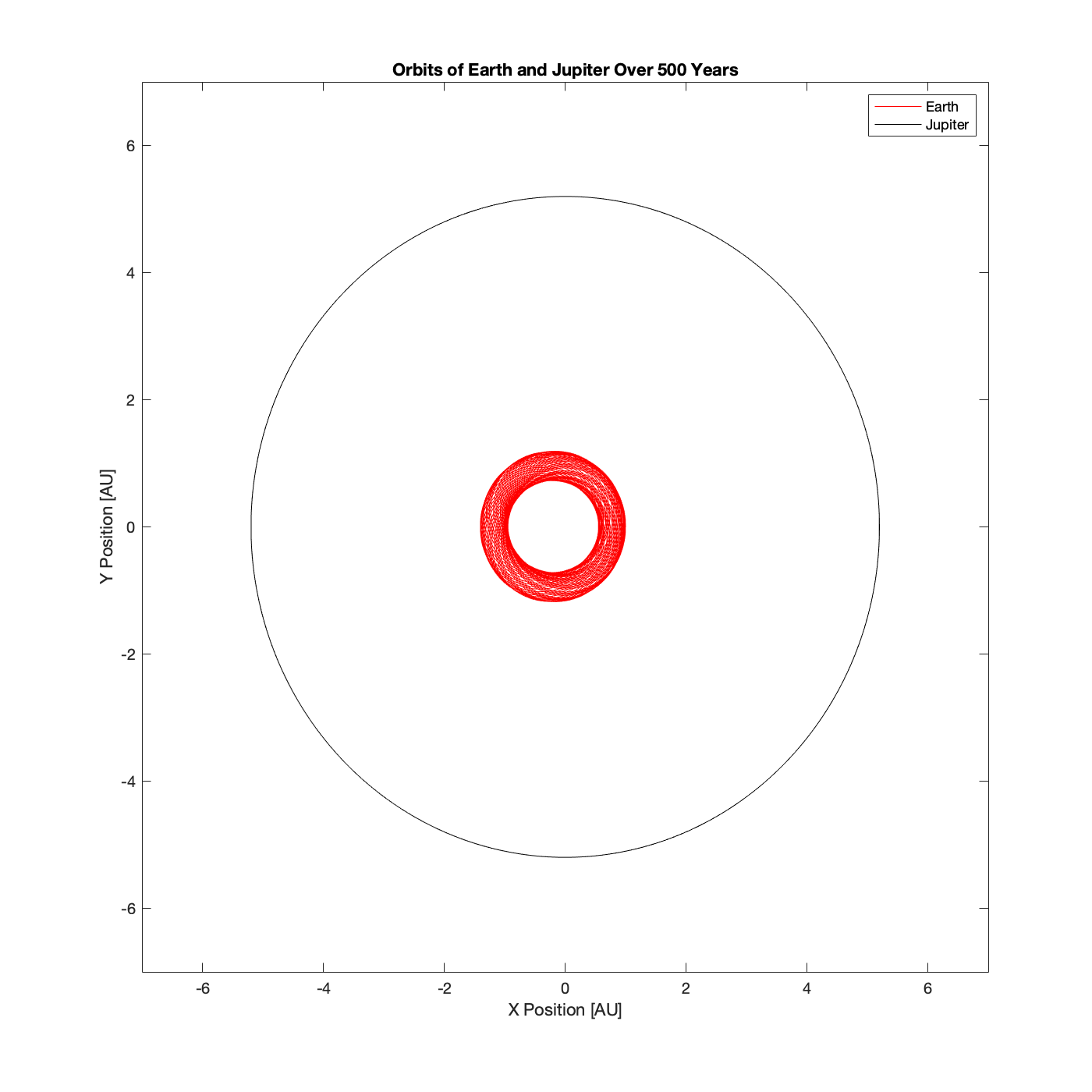
1 Jovian Mass

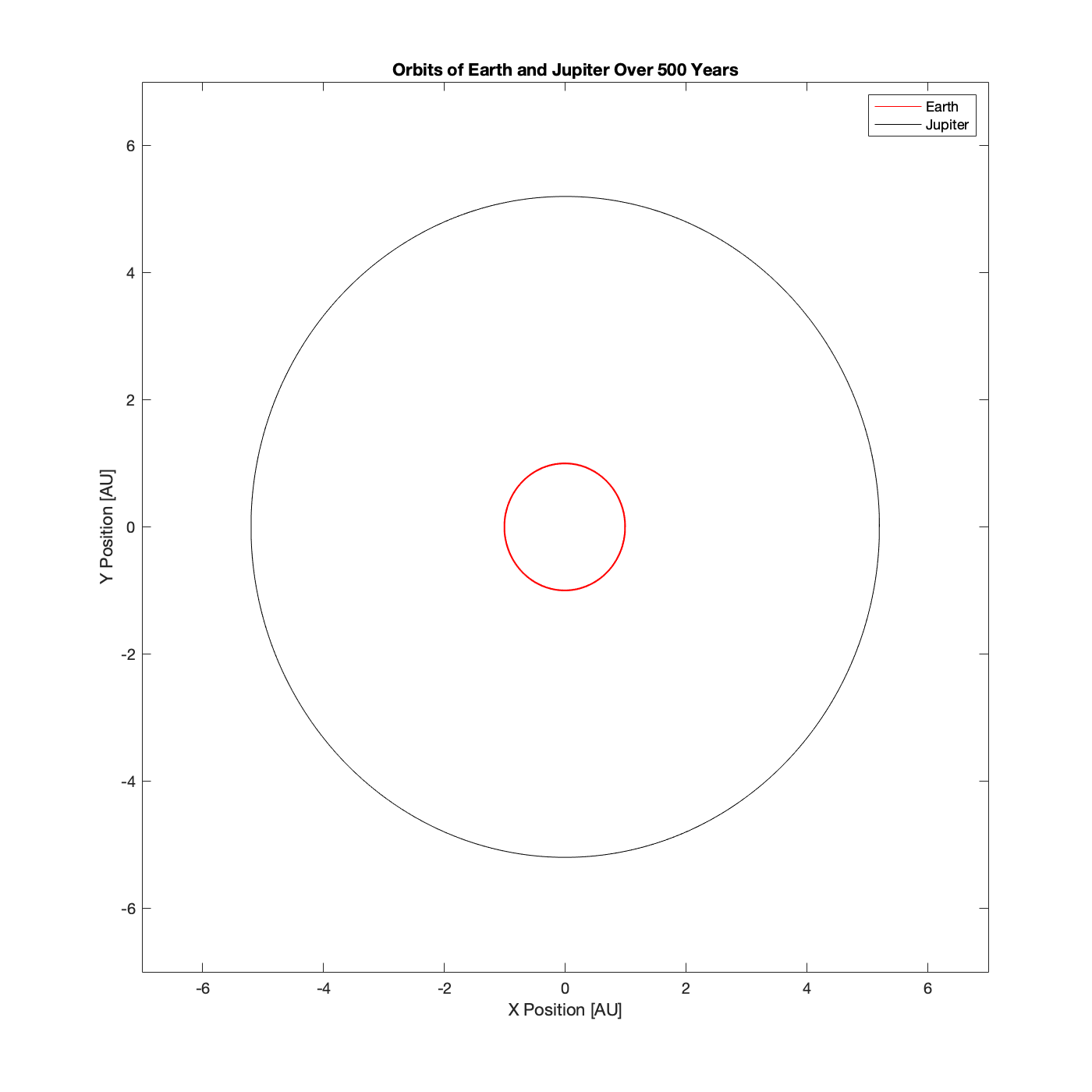
Mass of Planet = 1 Jovian Mass
Above is a simulation of the orbits of Earth and Jupiter where the mass of the Jovian planet is equivalent to 1 Jovian mass. This is the current state of our solar system, so this was mostly a check to see that the simulation was running correctly, as well as a way to have a result to compare future results to. The orbits remain completely circular and steady forever, with Earth staying at a distance of 1 AU and Jupiter staying at 5.2 AU, as expected.
10 Jovian Masses
Mass of Planet = 10 Jovian Masses
Above is a simulation where Jupiter’s mass is 10 times its standard value. There is almost no effect on Earth’s orbit here, so let’s increase the mass multiplier integer to 100.
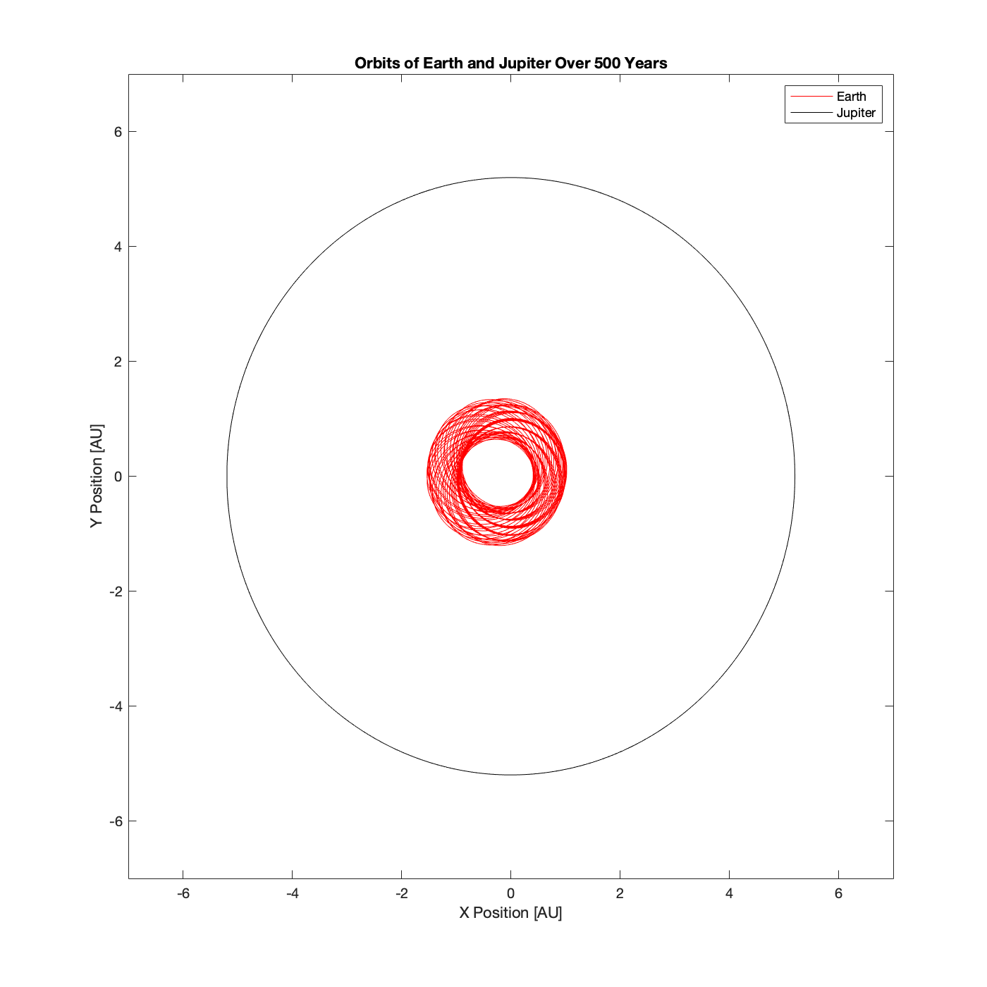
100 Jovian Masses
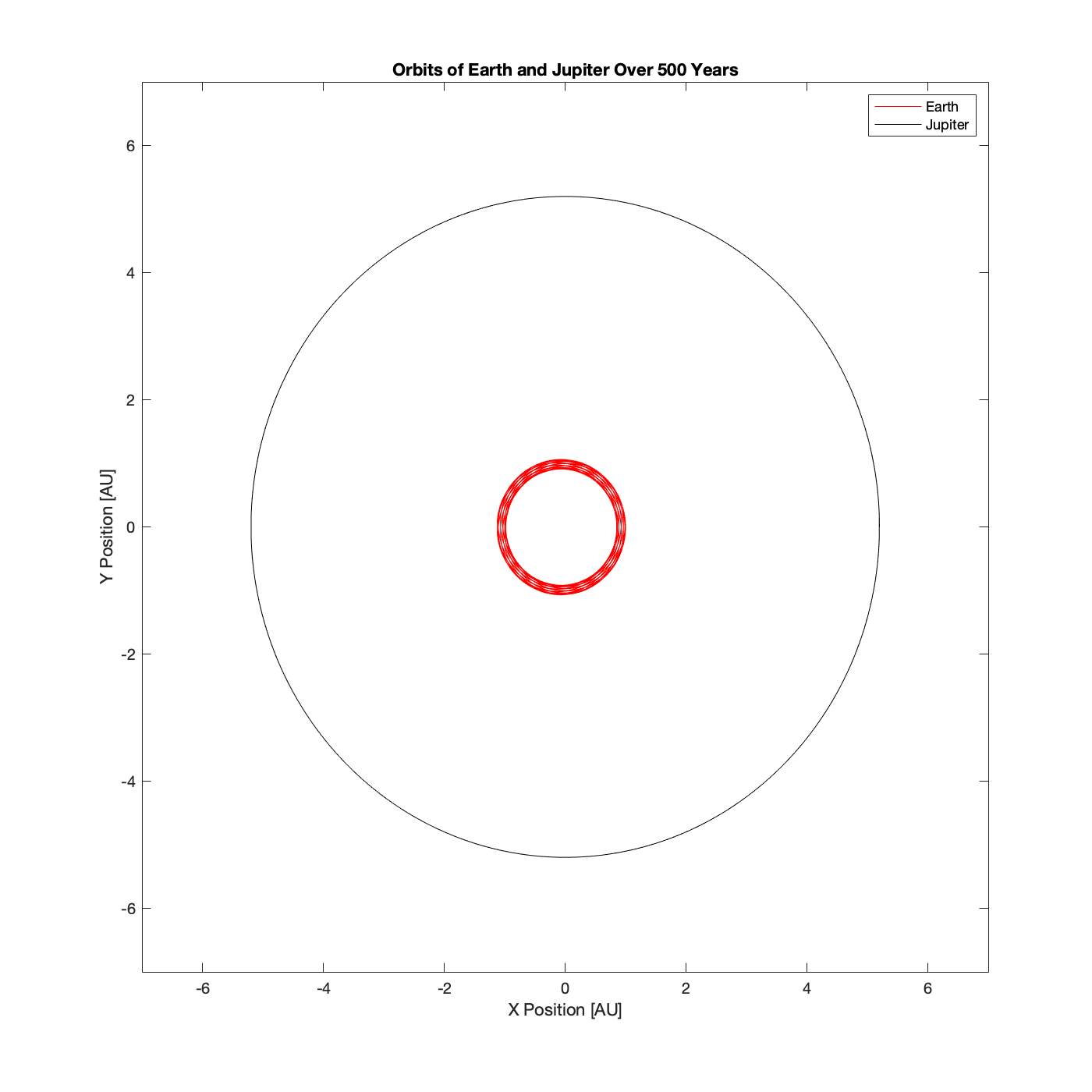
Mass of Planet = 100 Jovian Masses
Here, the Jovian planet is now 100 times larger than it is in our standard solar system. While Earth’s orbit is beginning to be affected, the effect is minimal and causes a slight oscillation in the otherwise perfectly circular orbit. Important (and astonishing) to note is that in this case Jupiter is already more massive than the least massive stars that we have discovered, and under the right formation conditions, would actually be a second star in the simulation rather than a second planet. Less astonishing, is the realization that this minimal effect makes sense since the force of gravity is inversely proportional to the square of the distance between the two gravitationally interacting objects, the effects of the Sun overpower the effects of the farther away Jovian planet. Clearly, it’s going to take a lot of mass to really affect Earth’s orbit, so going forward lets continue to use increments of 100 Jovian masses.
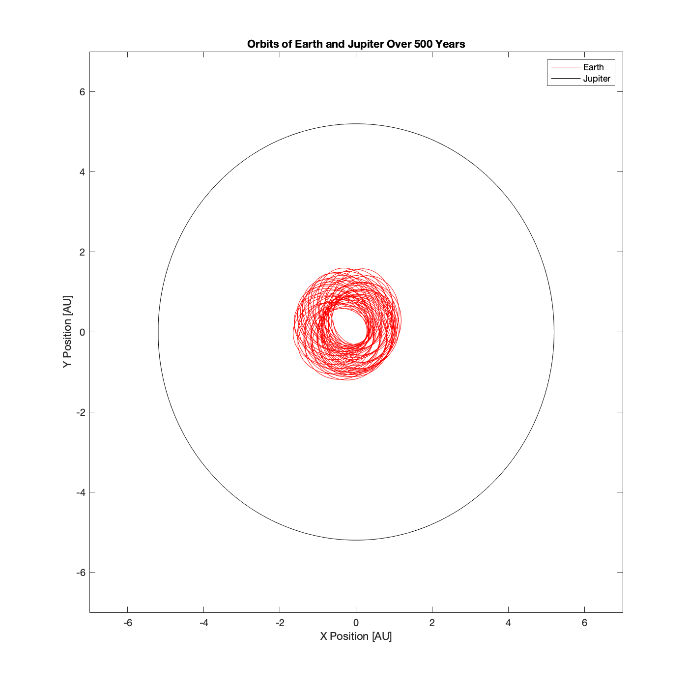
200 Jovian Masses
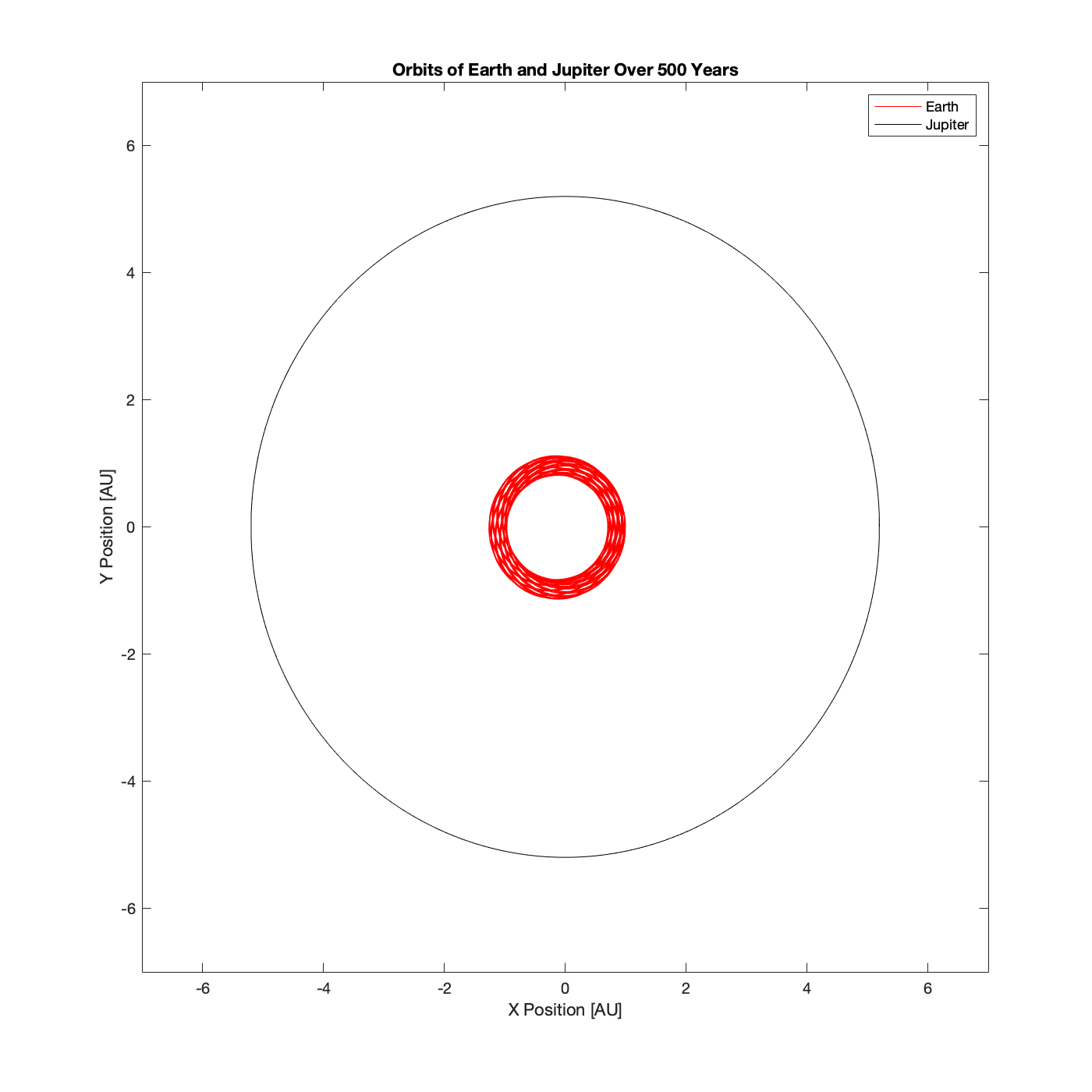
Mass of Planet = 200 Jovian Masses
At a planetary mass of 200 Jovian masses, we can observe the oscillations deviating from a perfect, constant circle more than before. However, Earth is still very much attached to the Sun, so let’s keep going until it isn’t.
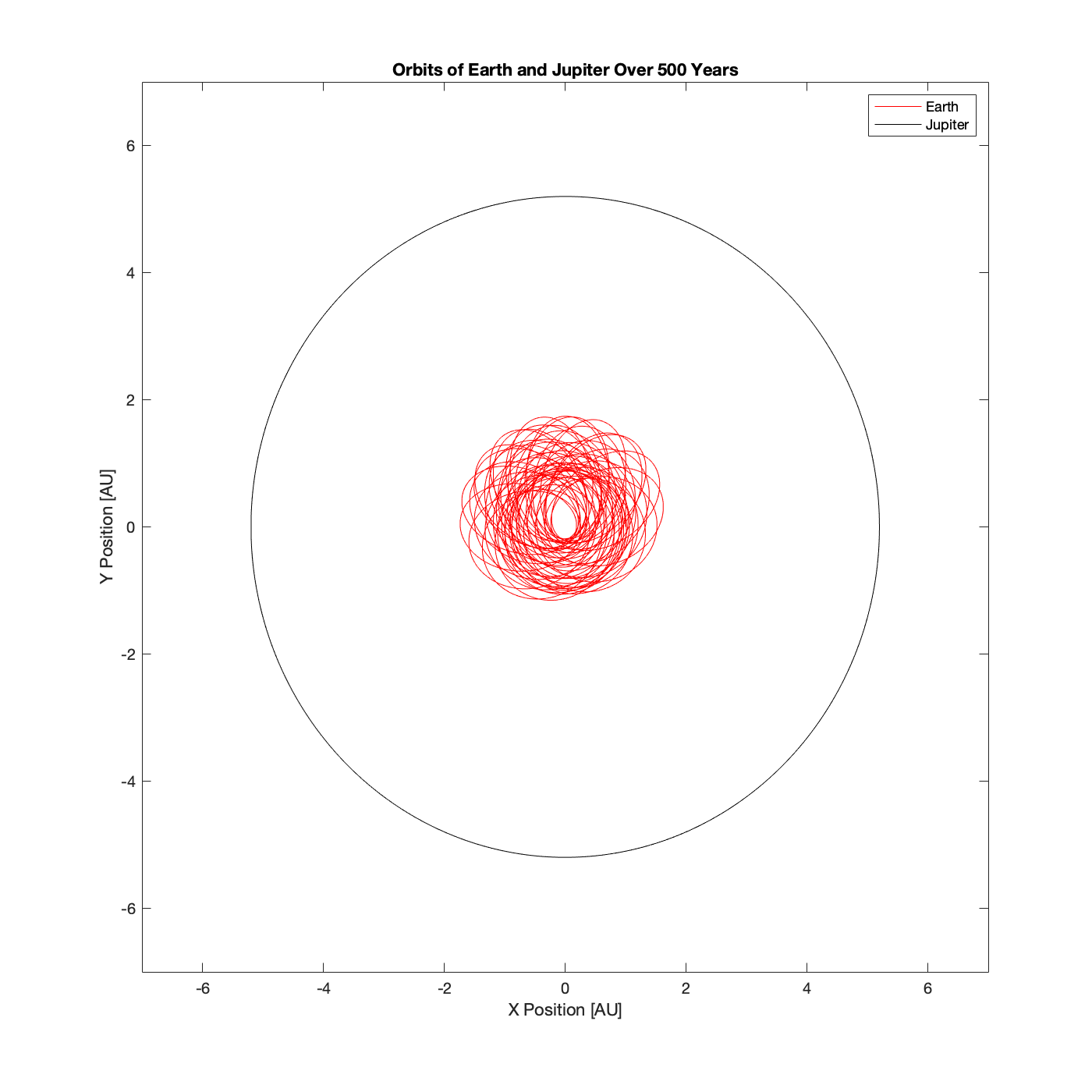
300 Jovian Masses
Mass of Planet = 300 Jovian Masses
At 300 Jovian masses, oscillatory motion is more pronounced than before.
400 Jovian Masses
Mass of Planet = 400 Jovian Masses
At 400 Jovian masses, Jupiter’s effect becomes more substantial.
500 Jovian Masses
Mass of Planet = 500 Jovian Masses
The trend continues for 500 Jovian masses.
600 Jovian Masses
Mass of Planet = 600 Jovian Masses
The trend continues for 600 Jovian masses.
700 Jovian Masses
Mass of Planet = 700 Jovian Masses
The trend continues for 700 Jovian masses.
800 Jovian Masses

Mass of Planet = 800 Jovian Masses
The trend continues (yes, still) for 800 Jovian masses.
900 Jovian Masses

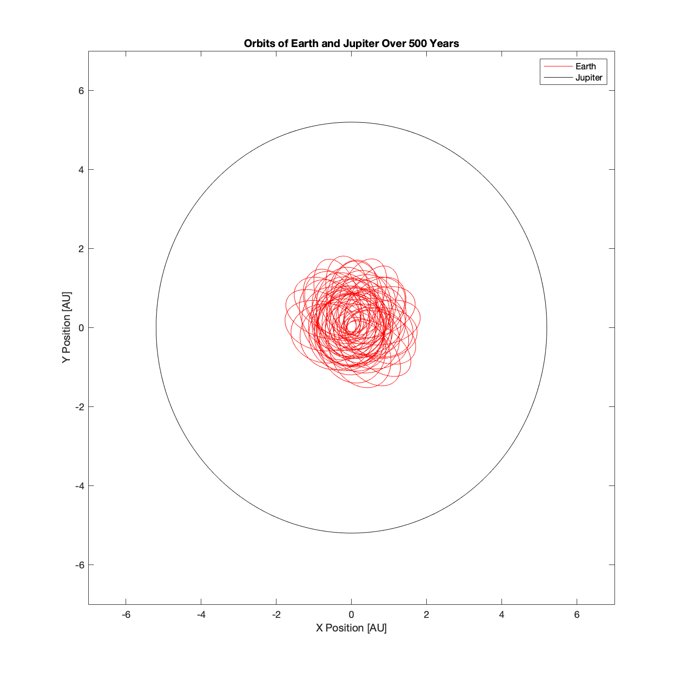
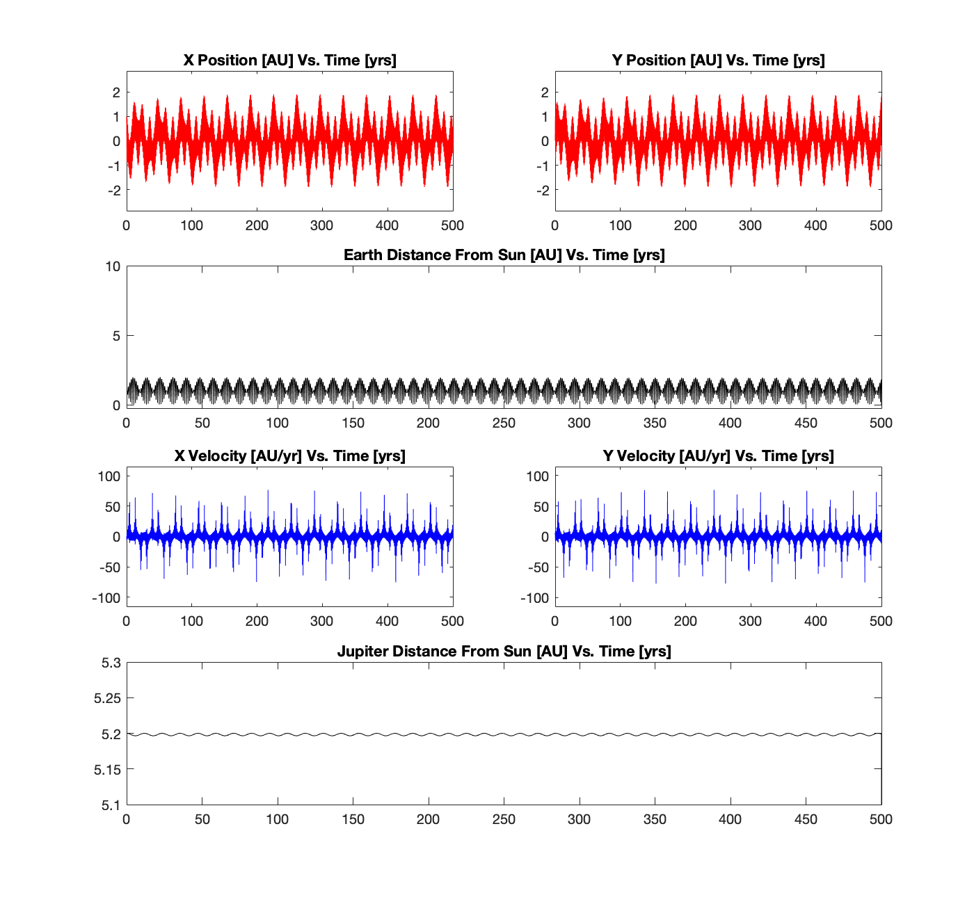
Mass of Planet = 900 Jovian Masses

Mass of Planet = 900 Jovian Masses
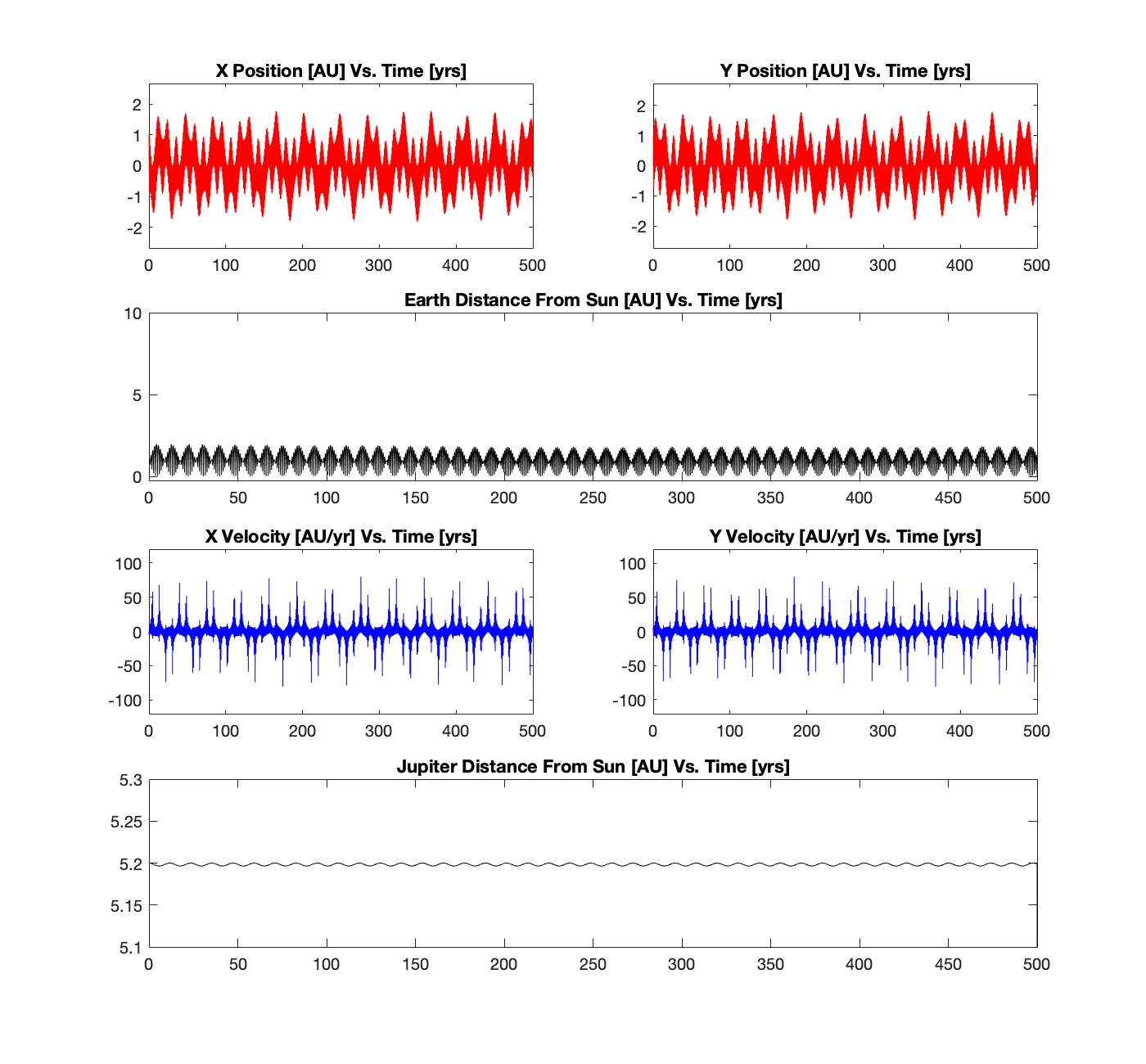
Still, at 900 Jovian masses, Earth can’t seem to let go of its connection to the solar system, but the amplitude of the oscillation has been and continues to increase, and it seems like we’re getting close to the ultimate goal: Earth’s ejection. To showcase the physics and beauty of this motion that is hidden by 500 years overlapping orbits, I have included plots of Earth’s x position, y position, x velocity, y velocity, and distance from the Sun versus time, as well as Jupiter’s distance from the Sun versus time.
After concern that I would never see Earth leave the solar system, hope was finally found between 900 and 1000 Jovian masses. For reference, our Sun is approximately 1048 Jovian masses, so Jupiter is distinctively in the mass range of stars at this point.
961 Jovian Masses (Last Consistently Stable Orbit)

Mass of Planet = 961 Jovian Masses
Mass of Planet = 961 Jovian Masses
Above is the last consistently stable orbit, which occurs at 961 Jovian masses.
962 Jovian Masses (Minimum Mass for Escape)
Mass of Planet = 962 Jovian Masses
Mass of Planet = 962 Jovian Masses
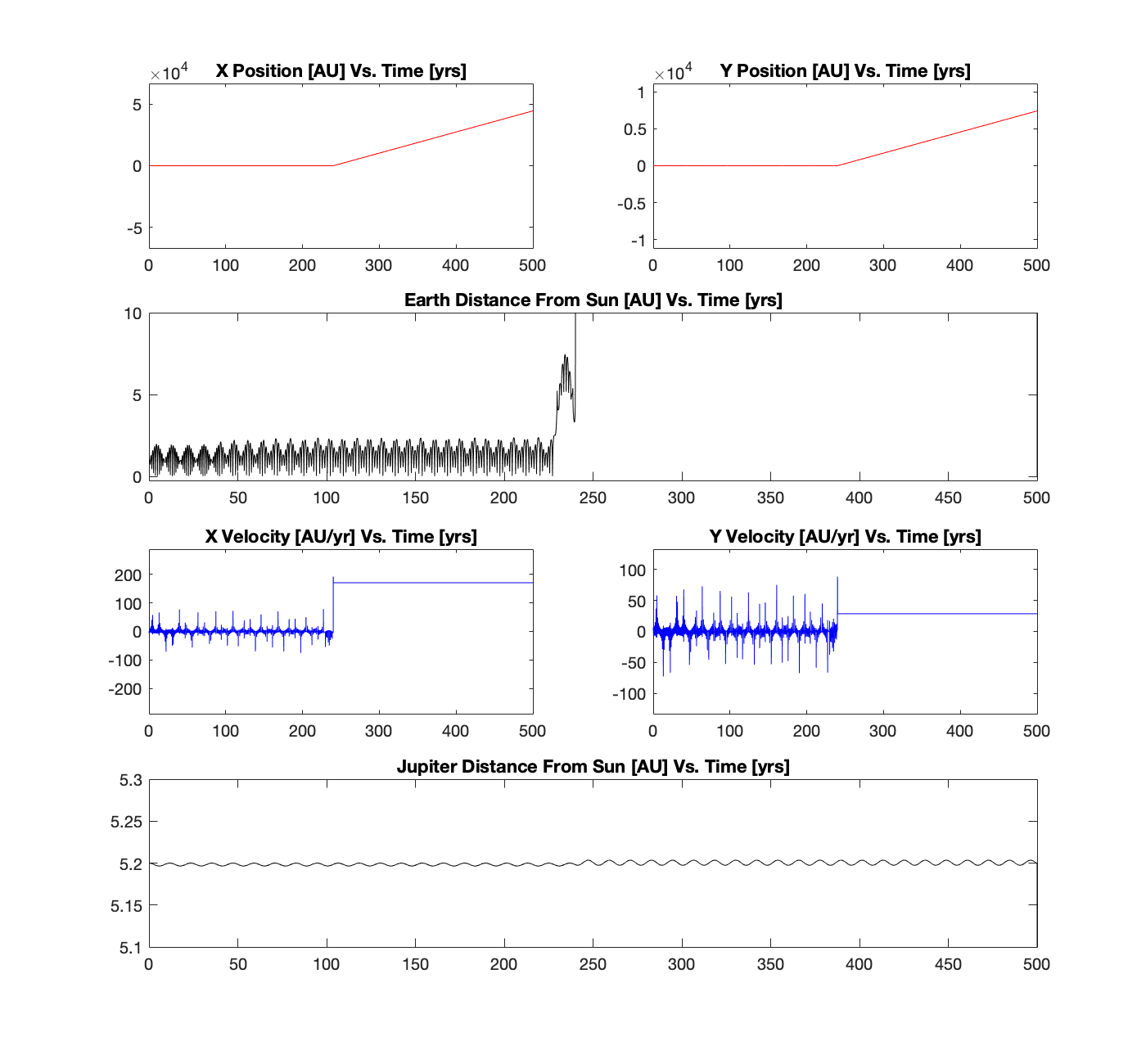
Above is the lowest planetary mass, 962 Jovian masses, that caused the Earth to be ejected from the solar system. Increasing by 1 Jovian mass from here results in a string of diverging solutions between 962 and 969 Jovian masses where sometimes Earth is ejected, and sometimes it remains stably in the solar system during this 500 year timespan. Ejection occurs around 220 years from the beginning of the simulation.
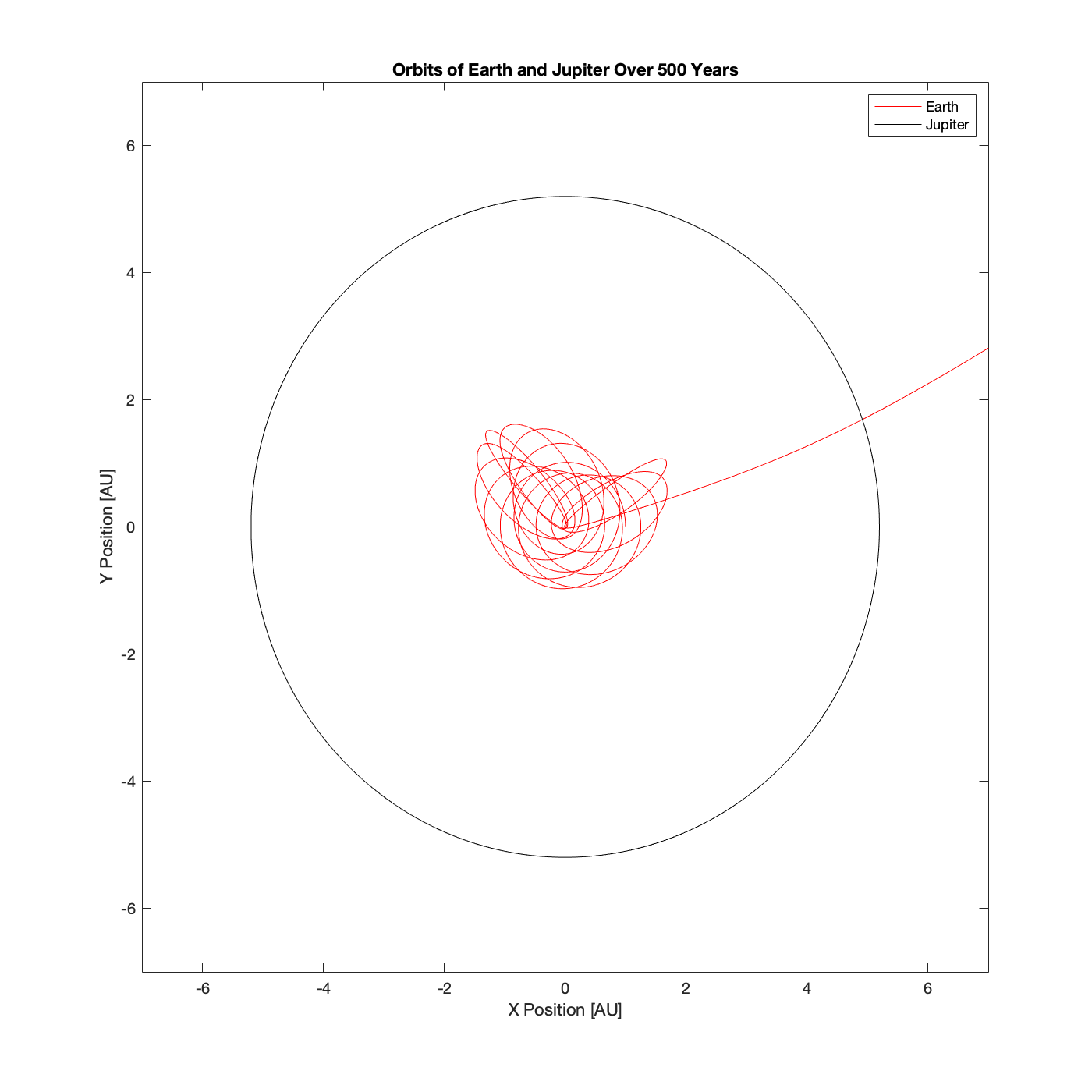
967 Jovian Masses (Random Cool Orbit)

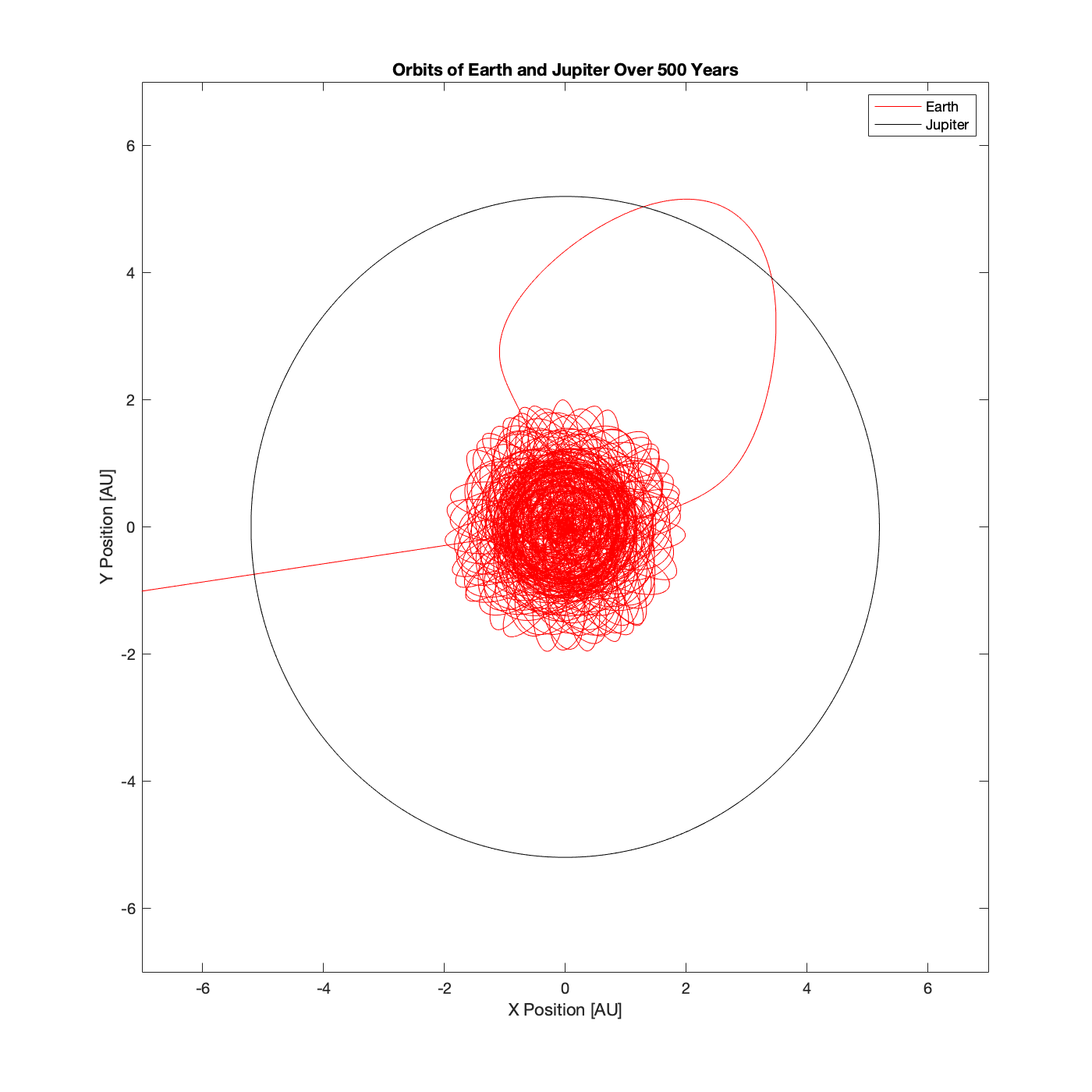
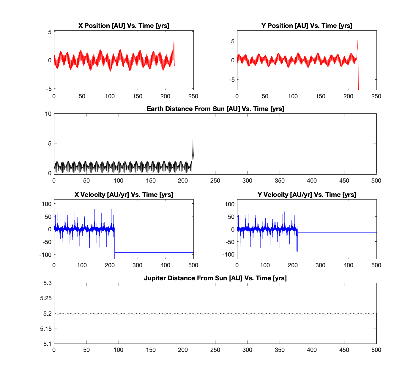
Mass of Planet = 967 Jovian Masses
Mass of Planet = 967 Jovian Masses
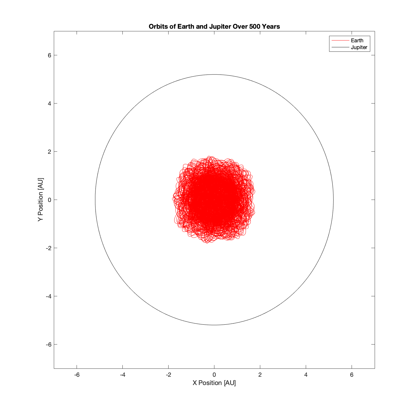
While at first this spatial map just was really fascinating to look at, I realized there were some interesting conclusions to be drawn. First, it is easy to trace the orbital path of Earth and Jupiter simultaneously around the time of ejection. ~240 years, and see how Earth has epicycles (small orbits) around the Jovian planet, becoming a temporary moon of Jupiter for about a Jovian year (~12 Earth years) before finally leaving the solar system with a nice gravity assist from the overwhelmingly massive Jovian planet. Additionally, this final, brief interaction seems to have affected Jupiter’s orbit! While up until this point, Jupiter’s distance from the Sun has predictably oscillated minimally (by about .01 AU) around 5.2 AU, this oscillation increases at ~240 years, when Earth finally leaves Jupiter’s and the Sun’s sphere of gravitational influence.
969 Jovian Masses (Maximum Mass to Stay)
Mass of Planet = 969 Jovian Masses
Mass of Planet = 969 Jovian Masses
As said before, the 960s present oscillating results – sometimes escaping, sometimes not. 969 Jovian masses seems to be the critical planetary mass limit above which Earth is guaranteed to be ejected within a simulation time of 500 years.
970 Jovian Masses (First Consistently Unstable Orbit)

Mass of Planet = 970 Jovian Masses
Mass of Planet = 970 Jovian Masses
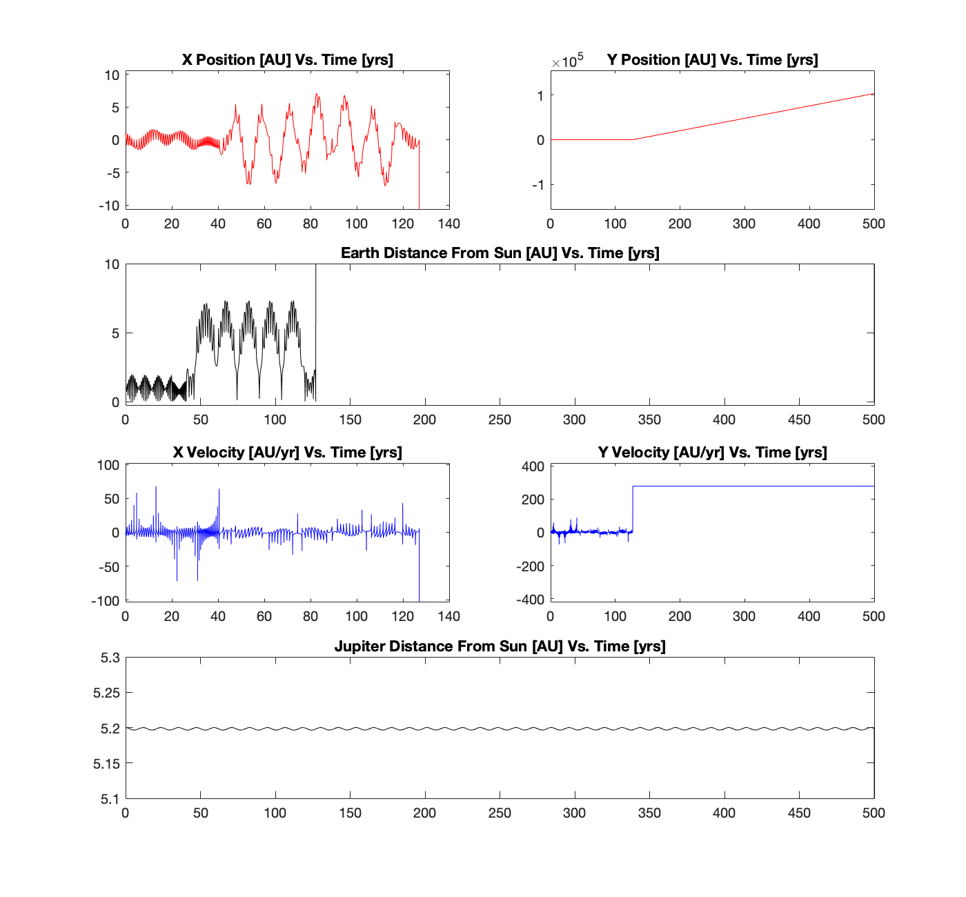
At 970 Jovian masses, we find the lowest mass value that guarantees Earth’s escape. At this mass quantity, escape occurs after about 120 years. All jovian masses greater than this result in escape as well. Interesting to note is that while it features similar epicycles (for several Jovian years) around the Jovian planet as seen at 967 Jovian masses, we do not see the same effect on Jupiter’s orbit as a result. Since it appears that this escape occurs when Earth is not surrounding Jupiter, the effect seen before was likely due to Earth being so close to Jupiter at its time of escape.
1000 Jovian Masses
Mass of Planet = 1000 Jovian Masses

Mass of Planet = 1000 Jovian Masses
As I continue to increase the mass of the Jovian planet, I see increasingly shorter escape times. At 1000 Jovian masses, Earth reliably leaves the solar system after about 15 years, barely more than one orbit of Jupiter. This trend continues with increasing mass.
Conclusions & Limitations
Ultimately, after many runs of this simulation, I conclude that the average critical Jovian mass for Earth’s escape is 965.5 ± 3.5 Jovian masses, found in the valley of oscillatory results (960s). Additionally, Earth’s semi-major axis, the distance from the star to the planet, never exceeds 2 AU.
Now, I will dissect some of the limitations or invalid assumptions of the simulation:
- The Sun is a fixed point mass. While approximating planets as point masses is fine, fixing the Sun’s position to not be affected by the gravity of the other celestial bodies is not. The effect is minimal for small Jovian masses, as the Sun remains containing nearly 100% of the mass of the solar system. However, the larger I made the mass of Jupiter, the more aphysical the solution became since the Sun would obviously be moving considerably – especially once the mass of Jupiter began to rival that of the Sun itself.
- A step size of 10^-4 is good enough. While a step size this small is very accurate, further decreasing the step size actually gave results that conflicted with those obtained using the decided step size. I unfortunately couldn’t feasibly conduct the project this way due to the long computational time required for the slight increase in accuracy.
- Earth and Jupiter have basically circular orbits. While this is true, even a negligible deviation from a perfectly circular orbit would likely have dramatic effects after 5 million iterations, as is the case in this simulation.
- The Euler-Cromer method is sufficient. As addressed before, the Runge-Kutta method would have been more accurate and more useful for me.
Sources Cited
- https://nssdc.gsfc.nasa.gov/planetary/factsheet/jupiterfact.html
- http://urminsky.ca/wp-content/uploads/2016/08/lecture_8.pdf
- https://www.researchgate.net/publication/281108779_Numerical_Integration_Techniques_in_Orbital_Mechanics_Applications
- http://coffee.ncat.edu:8080/Flurchick/Lectures/StellarModeling/Section4/Lecture4-3.html
