Overview
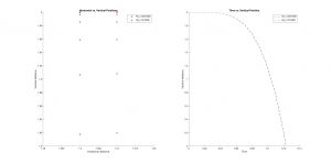
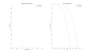
This project aimed to simulate the viscous drag forces that occur when a ball falls in fluids with different densities and viscosities, resulting in different Reynolds numbers. In this case, there are two graphs produced. The first shows the ball falling in the medium in phase-space. The second shows the vertical distance traveled by the ball in time. The ball falling in the fluid with the larger Reynold number should take a longer time to fall because the drag forces on the ball are greater. Fluids include both liquids and gases.
Reynolds numbers determine the type of flow the fluid will make. When Re<<1 the fluid follows Stoke’s Law. When Re>>1 the fluid does not,it follows the Navier-Stokes equations. The Reynolds number is a proportion of the inertial forces to the viscous forces, Re = inertial/viscous.
Motivations
While I studied abroad, I took a fluid dynamics class that covered the Navier-Stokes equations and complicated geometries of objects moving in fluids. The most basic geometry is a sphere in 3D and a circle/disk in 2D. I wanted to be able to visualize and create a code that could interpret various inputs for fluids and produce a 2D plot of the motion. It proved more difficult to do than initially thought because I do not have a solid background in fluid dynamics, just that one course. As a result, I referenced derivations for the Navier-Stokes, but most were more complicated than the 2D system I wanted to model. I referenced my notes from the course too and YouTube videos from MIT.
Figures (click on the images to make them larger)
Figure 1. The parameters of this plot are those of water and honey at room temperature (20° C). The viscosities are 1.0 (Pa s) and 1.36 (Pa s) and the densities are 0.7978 (kg/L) and 7.20 (kg/L) respectively. The ball travels slower in the honey, Re2.
Figure 2. The parameters for this plot are viscosities of 32 (Pa s) and 400 (Pa s), densities of 20 (kg/L) and 75 (kg/L), and kinematic viscosities of 1.6 and 5.33, respectively. The Reynolds numbers are displayed on the plots. The ball moves slower in the larger Reynolds number fluid.
Fluid Mechanics Physics
The above equations are the Navier-Stokes equations in 3D for cartesian coordinates. For the 2D version that I used, the z-direction components are removed. These equations are only used for when Re>>1, for high Reynolds numbers. Because the Navier-Stokes equations can only be solved for very specific cases I simplified the process by using the drag equation,
and then solved Newton’s second law for the vertical and horizontal directions, and formulated the kinematics equations. Buoyancy forces were ignored. This is a different case than than when Re<<1.
When Re<<1, the system follows viscous drag using Stoke’s Law
From here you can solve Newton’s second law and formulate the kinematic equations again. Stoke’s Law only works for these cases, otherwise Navier-Stokes and the drag equation are used. Buoyancy forces were ignored here too.
Results
Computational fluid dynamics (CFD) is a growing and complicated field of both mathematics and physics. The program I developed is part of the general sphere of CFD but not close to the type of programs are used and developed. CFD is used to simulate airplane designs, model the way fluids flow around objects. My program has some bugs because of the simplifications I used for the equations. By using an adapted version of the Navier-Stokes equations, not all parameter values work correctly with the model. For the many combinations of inputs, however, the larger Reynolds number fluid produces a slower movement in the fluid.
Conclusion
In the future, I would like to fix the bugs caused by the simplifications and possibly create a program that uses the Navier-Stokes equation in its full 3D form. If possible, it would be useful to have a GUI for the program because that would allow the user to more easily see the differences in the motion when the viscosities and densities of the fluids are changed. Perhaps adding more than two fluids to the model as well as making the visualization as a movie and not stagnant plots.
References
http://soliton.ae.gatech.edu/labs/windtunl/classes/hispd/hispd06/ns_eqns.html
http://www.personal.psu.edu/wzl113/Lesson%20Plan.htm#GF
http://scienceworld.wolfram.com/physics/StokesVelocity.html
https://www.grc.nasa.gov/www/k-12/airplane/nseqs.html
https://www.grc.nasa.gov/www/k-12/airplane/reynolds.html


