4 Body Orbital System
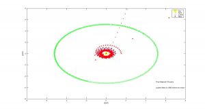
My model of Jupiter, Mars, and the Earth orbiting the Sun can be used as a tool for educating people about planetary motion. The planets have maintained their orbits for billions of years, but this model seeks to prove their stability and test under what conditions their orbits might become unstable. By gradually changing the mass of Jupiter, we can see that it is not until the planet’s mass is 1000 times more than its current weight that it would begin to affect the orbits of Mars and Earth. At this extremely increased mass, The Earth and Mars both exhibit unstable behavior. This model is not only interesting to those who study astronomy, but can be informative and reassuring of the Universe’s stability for those with no knowledge of the subject.
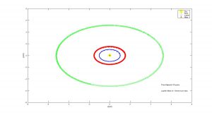
Physics and Astronomy often cause students a lot of anxiety. These subjects are not usually intuitive and can intimidate students, resulting in very few people studying the subject past high school.[1] This unfortunate occurrence must be minimized and graphical teaching tools can be an effective way to engage students. Presenting a visual representation of the often unobservable processes studied by physicians and astronomers is invaluable to a struggling student. Astronomy is inherently a visual subject and it makes sense to model computationally phenomena that may take too long to study physically. With a computational model you can map the progress of a planet for years in a matter of seconds. My model maps the orbits of Jupiter, Mars, and Earth for 20 years and includes a legend and text that makes it easily interpreted. My hope is that this model will help to illuminate the effects of planetary gravitational pull to beginning astronomy students.
Graph 1: This graph shows the orbits of Earth, Mars, and Jupiter after 20 years when Jupiter is at its normal mass.
Graph 2: The orbits after the mass of Jupiter has been increased by a factor of 1000.
These graphs are made by building equations from Kepler’s laws that make each planet sensitive to the gravity of all other planets in the system. This means that each planet will have four equations to solve for its velocity and position. The following shows the velocity equation for the x direction of the Earth.
vxE(i+1)=vxE(i)-(4*(pi^2)*xE(i).*dt)/(rE(i).^3)-4*pi^2*(J/S)*(xE(i)- xJ(i))*dt/rEJ(i)^3-4*pi^2*(M/S)*(xE(i)- xM(i))*dt/rEM(i)^3;
Each velocity equation must account for the mass and gravitational pull of the surrounding planets and can be done by manipulating Kepler’s laws. These equations should then be iterated using the Euler-Cromer Method.
The Euler Cromer Method is usually the best method to model oscillatory motion. In my first draft of this code, I modeled the lone Earth around the Sun. Because of an error in my equation, the Earth’s orbit was not elliptical. Upon doing further research, I attempted a 2nd Order Runge-Kutta model which proved too complicated to use when finishing the entire system. [2] I eventually was able to successfully use the Euler-Cromer Method which now perfectly models the orbital motion.
Conclusion:
This project was able to successfully build a teaching tool that would be really easily used in a classroom setting. The animation makes the model interesting to students and the year counter lets you know exactly when Earth and Mars would shoot off into space. While the unstable behavior only occurs under extreme circumstances, it is still an excellent lesson on the stability of the solar system. In the future, I would love to add more planets to the system, but I fear that the length of my equations and the number of matrices I would need to create would slow the computing time considerably. When I added Mars to the system, I had to create another 7 matrices and my equations increased sizably in length. In addition, the perihelion of mercury is more complicated to calculate and might pose a problem. Despite these potential issues, a system in which all 8 planets are represented would extremely enhance the model and its educational value.
Resources:
- Grim, Nancy. A Force Concept Correlation Study with Instructional Methods, Anxiety, Perceptions of Difficulty and Student Background Variables. 1999. 11 Dec. 2016 <http://eric.ed.gov/?id=ED438164>.
- Giordano, Nicholas J., and Hisao Nakanishi. Computational physics. Pearson Education India, 2006.


