Overview:
The stated goal of this project was to create a set of simulations to be used in an educational environment to better understand the orbital dynamics of a binary star system by plotting, in 2-D, the x and y positions of the celestial objects within the system. This project was split up into four subsections, or subprograms within the program. The first subprogram considered a simple binary star system, the second a system with stars that had different velocities, the third a system with stars that had low velocities, and the fourth a simple system with a planet orbiting one of the stars. We deviated slightly from our project plan because we were unable to explore the effects of mass on the orbits of the stars; this was because of an issue that arose within our model, prohibiting us from being able to accurately assess the effects of mass. Here, we present our results and conclusion of our project. The method section has been omitted, but can be found within our program for each subprogram.
Results:
All of our subprograms self-generated data, based on some initial parameters, and plotted that data on graphs for N iterations. We have attached our graphs here in the form of clickable GIFs. The number of iterations N is responsible for the accuracy of our orbits. In our programs, we use low values for N to obtain semi-accurate orbital data without expending too much computational power or too much time. This is why our orbits may not seem to completely line up; if we increase N to around a thousand or fifteen hundred, then we will see that the orbits will line up quite well. It is important to note that the dots are representative of the velocities of the celestial objects. If there is a cluster of consecutive dots, that indicates that the celestial objects are moving with constant velocities; however, if consecutive dots are far apart, that indicates that the celestial objects are moving with increasing velocity. Additionally, the units used here are not standard units; our position units are in AU, our velocity units are of the form 2πAU/yr, and our mass units are in kg. Below we discuss the results of each subprogram.
I. Simple Binary Star System:
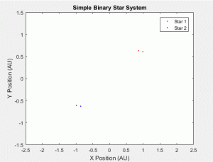
For our first subprogram, as mentioned previously, we tried to generate a simple binary star system. Our initial parameters were as follows:
For star 1, x = .72, y = .64, V_x = 2.42π, V_y = 0, and M = 5*10^30.
For star 2, x = -.72, y = -.64, V_x = -2.42π, V_y = 0, and M = 5*10^30.
Note that our masses for our stars here are equal (5*10^30 kg). We compared our results, shown in Figure 1.1, to some simulations online, which also had the stars being of equal mass: 1 and 2. Our simulation seemed to be in line with these results. We can also understand why our result makes sense using our knowledge of physics. First, we must consider the following equation:
 This is the equation for gravitational force between two celestial objects with masses of M_S and M_E. Since our binary star orbit is supposed to be stable, F=F_G=ma. If the objects are close together, then the gravitational force between them is maximized, but because this has to be equal to ma, acceleration must increase since mass cannot be changed. This increase in acceleration is the reason for the increase in velocity. Similarly, if the objects are far apart, then the gravitational force between them is minimized and we expect acceleration to decrease, so the velocities of the objects will approach a constant value.
II. What if the Stars have Different Velocities?
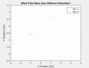
Once we were able to generate the simple binary star system, we wanted to see the effects on the orbits due to a change in velocity. For this program, our initial parameters were:
For star 1, x = .72, y = .64, V_x = 2.6π, V_y = 0, and M = 5*10^30.
For star 2, x = -.72, y = -.64, V_x = -2.42π , V_y = 0, and M = 5*10^30.
We increased the V_x of star 1 to 2.6π and kept star 2’s V_x at -2.42π, the same as in subprogram 1. The results can be seen in Figure 1.2. It is, however, important to note a flaw on our method. Namely, we assigned mass to the common barycenter of the stars. This was initially useful to stabilize the orbits of the stars, but as seen here, it makes it so that the orbit star 2 is not affected by that of star 1. We did, however, expect the orbit of star 1 to be more elliptical with a higher velocity because an increase in velocity would mean that the star would be getting closer to its escape velocity, at which point it would move in a straight line.
III. What if the Stars have Low Velocities?
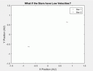
Next, since we were unable to consider changes in mass, we considered the case where the velocities of both stars were very low. For this program, our initial parameters were:
For star 1, x = .72, y = .64, V_x = 1.5π, V_y = 0, and M = 5*10^30.
For star 2, x = -.72, y = -.64, V_x = -1.5π, V_y = 0, and M = 5*10^30.
Note the decrease in velocity from 2.42π and -2.42π to 1.5π and -1.5π for star 1 and star 2, respectively. The result we obtained is shown in Figure 1.3. This result is rather interesting because it seems that the orbits of the stars are moving in a counterclockwise direction through space. However, this orbit is not stable because, after some time, the stars would both escape the system (we know this because we ran this for many iterations before, but did not display it here). We attempted to find a simulation online for comparison, but we were unsuccessful in doing so. However, given that this is built on the program of the simple binary star system, which we know is fairly accurate, we can assume that this may also be a fairly accurate representation.
IV. Simple Binary Star System with a Planet:
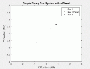
This subprogram is the one that we built up to using our previous problems. With a good grasp of the flaws of our system and the orbital dynamics of a simple binary star system, we introduced a planet. Below are our initial parameters:
For star 1, x = .72, y = .64, V_x = 2.42π, V_y = 0, and M = 5*10^30.
For star 1’s planet, x = .3, y = .3, V_x = .09π, V_y = 0, and M = 2*10^24.
For star 2, x = -.72, y = -.64, V_x = -2.42π, V_y = 0, and M = 5*10^30.
The result of our program can be seen in Figure 1.4. It is important to note the initial behavior of the planet. Initially, the planet is assisted by the gravitational force of its host star (since their initial velocities are in the same direction) and moves very quickly outside of the system, but because of the gravitational force of its host star, it is then pulled into an orbit around it. The behavior of the planet is interesting because, as its host star moves, it attempts to stay in orbit by moving along with it. This was to be expected. However, after some time, the planet exits the system. This indicates that this orbit is highly unstable. Although, much time was spent attempting to find a stable orbit with no success. This could explain why we were also unable to find a simulation for comparison – it seems extremely rare or difficult for a planet to be in a stable orbit in a binary star system. Although it must be noted that we had only taken into account the gravitational force on the planet by its host star; previously, we experienced crashes of MATLAB when we attempted to consider the gravitational force of both stars on the planet.
Conclusion:
Referring to our project plans, we were able to achieve most of what we aimed to do. We also believe that this set of simulations can be useful in an educational environment for students. However, because of our model, the only thing we were not able to accurately assess was the effect of mass on a binary star system. Although there are already some interactive simulations online, such as this one, that do so. We experienced a lot of difficulty in building our initial model because we were attempting to replicate an example outlined in Computational Physics. However, we managed to create a good base program to explore further simulations. If we can continue to build on this model, we may consider working out the kinks with taking into account the gravitational force of star 1 and 2 on star 1’s planet. Additionally, it would be interesting to consider multiple planets in different orbits around this binary star system.
References:
“Binary Star.” Wikipedia. Wikimedia Foundation, n.d. Web. 28 Nov. 2016. <https://en.wikipedia.org/wiki/Binary_star#Center_of_mass_animations>.
Fix, John D. “Interactives.” Interactives. N.p., n.d. Web. 28 Nov. 2016. <http://highered.mheducation.com/sites/0072482621/student_view0/interactives.html#>.
Giordano, Nicholas J., and Hisao Nakanishi. Computational Physics. 2nd ed. Upper Saddle River, NJ: Prentice Hall, 2006. Print.
Zingale, Michael. “Introductory Astronomy Animations (and Figures).” N.p., n.d. Web. <https://zingale.github.io/astro_animations/>.


