At this point in the Spring semester students in Geog/Esci 224: GIS begin to ramp-up work on their final projects, and many of them are looking for data related to a topic or question they will be mapping and analyzing in GIS. While there’s a lot of data to be found, getting familiar with it once you have it – enough to make some useful and interesting maps – can take some time. Different data providers create and organize their data in different ways, which can be difficult to understand at first. Users should also understand something about the methods used to collect and assemble the data. This may have important implications for how the data could and should be used.
Students often want to work with demographic and socioeconomic data, and one of the richest sources of this type of data (at least, in the US) is the U.S. Census and American Community Survey (ACS) data. The purpose of this article is to provide students with a brief introduction to the U.S. Census and ACS GIS data available, and how and where to get it.
Various pieces of information in this post is borrowed from pbc Goegraphic Information Services. Other sources are credited where appropriate. As always, if you need help with this data or any other GIS and mapping help, feel free to contact me at necurri@vassar.edu.
Census data basics
The U.S. Census provides information on sex, age, date of birth, race, ethnicity, relationship and housing tenure. The ACS provides more detailed socioeconomic information. In order to protect the confidentiality of individuals, the U.S. Census Bureau releases only summary statistics from the U.S. Census and ACS for geographic areas, such as blocks, block-groups and tracts.
- Census Blocks – In urban areas, census blocks conform approximately to what we think of as city blocks. At this fine level of geography, the U.S. census only releases a subset of the data short-form questionnaire.
- Block Groups – These areas are supposed to contain approximately 1200 people, but the actual count of people per block group varies widely. All of the short and long-form data is summarized at the block-group and tract level. Between 1970 and 2000, the U.S. Census Bureau used two questionnaires. Most households received the short-form questionnaire asking a minimum number of questions. A sample of households received a long-form questionnaire that included additional questions about the household. The 2010 Census had just one questionnaire consisting of ten questions. (View questionnaires from past years in the wonderful History section of the U.S. Census Bureau’s website > through the decades > questionnaires.)
- Tracts – Tracts are larger than block groups.
Census and ACS information is also aggregated at the County and State level (though not every statistic is provided at every level). Here’s an illustration from Esri about the relationship between the geographies at which census and ACS data is aggregated:
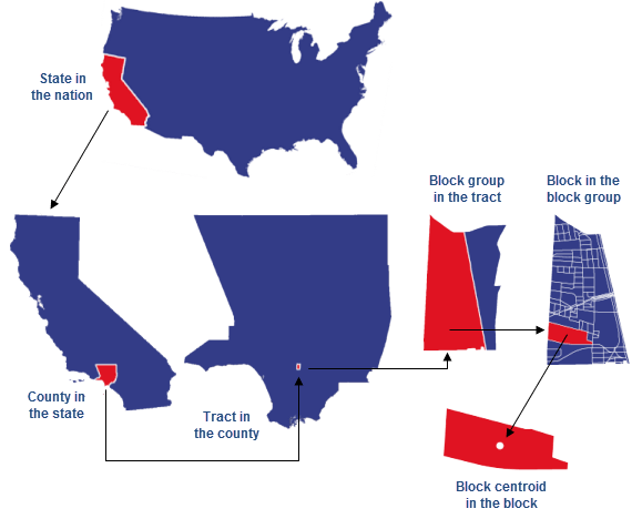
Census geographies: blocks, block groups, tracts, counties, and states. Source: Esri
Census and ACS data is also aggregated at other geographies, such as zip code, congressional districts, tribal areas, school districts, and others. You’ll see that later on in the download page (link below). Whether or not you should map or analyze data at these geographies depends on your research question. Consult with your professor or me (necurri@vassar.edu) for guidance if needed.
Previously, the only way to map and analyze Census data in GIS software was to download the TIGER shapefiles for the different geographies at which the data was tabulated (block, block group, county, state…), then navigate the American Factfinder website to find and download the demographic data you want in tabular format, then modify the tabular data so that it is ArcMap-friendly and can be joined to the TIGER shapefiles, then join and export the data for your area(s) of interest to new shapefiles or geodatabase feature classes. You can still do this if you know exactly the statistic you’re looking for. This excellent tutorial from the Tufts Data Lab GIS Center will guide you through this process.
However, if you want to just get your hands on some data quickly and start exploring some of the different demographic variables you can map and analyze, there’s an alternative. Pre-staged data sets are now available at various Census geographies (block, block group, tract… etc.) with much of the demographic data collected in the U.S. Census and ACS. These are provided as GIS data sets with “ready to join” tables, aggregated at the same geography as the GIS data. The only caveat is that you get almost ALL of the data aggregated at each geography. That’s a LOT of columns to sift through to find what it is you want to map or analyze. But, this is a potentially useful data set to use to explore what demographic and socioeconomic data is available, and to try mapping several different statistics in your study area before deciding on what variables you want to work with.
Before jumping head-first into that data, though, let’s take a minute to get a little background on the ACS data.
American Community Survey (ACS) basics
The U.S. Bureau of the Census has been collecting demographic information since 1790, when it was stipulated by the U.S. constitution that information about households be collected every decade from then on. (This is why it is often referred to in the documentation as the Decennial Census.) The most recent census was taken in 2010. Prior censuses were taken in 2000, 1990, 1980, and so on back to the first census in 1790. The information collected in the Decennial Census questionnaire (a.k.a. short form) is used to determine allotments of governmental resources, including congressional representatives and education funding. Between the years 1940 and 2000, the U.S. Census Bureau also sent out a longer form questionnaire (a.k.a. long form) to a smaller sample of households (1 in 6). The long form survey collected information such as Income, Occupation, Housing Stock, Rent and Mortgage, Commuting behavior and many others. This long form survey was discontinued for the 2010 census and replaced with the American Community Survey, which is collected every year but with a much smaller sample size.
ACS provides estimates based on 12 months of collected data (1-year estimates), 36 months (3-year estimates), or 60 months (50-year estimates). This sampling method leads to a certain amount of error. In general, the precision of the estimates increases with increasing periods of sample data. The table below outlines the distinguishing features of the 1-year, 3- year, and 5-year ACS estimates, and why you might choose to use one over the other. (Note: ACS 3-year estimates have been discontinued, but estimates for previous years will remain available.)
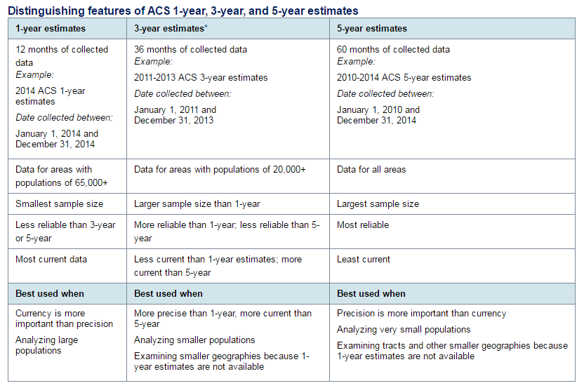
Distinguishing features of ACS 1-year, 3-year, and 5-year estimates. Source: U.S. Census Bureau
How to get the data
The pre-staged data sets are available on this page of Census website: TIGER/Line with Selected Demographic and Economic Data. Note that the ACS data is provided separately from the Census data. Note also that only 5-year ACS data is provided, and only in geodatabase format. If you want 1 or 3-year ACS data, you’ll have to do it the other way (see the aforementioned Tufts tutorial). The Census data is provided in either shapefile or geodatabase format.
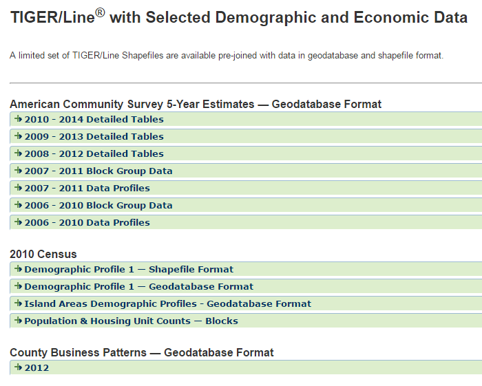
Download page: TIGER/Line with Selected Demographic and Economic Data
Here’s a brief overview of the datasets available:
2010 Census
Population & Housing Unit Counts – Provided at the block level geography as state-wide datasets. This is the most basic data to look at: a simple tally of the number of individuals and households in each block.
Demographic Profile 1 (shapefile or geodatabase format) – Provides more detailed information, and is available at various geographies. After downloading and viewing the data in ArcMap or ArcCatalog, you’ll notice the attribute column names are a little cryptic. Here’s a look at the county-level shapefile attribute table. (I’ve hidden some of the columns and can only show a few within the space of a screenshot.)
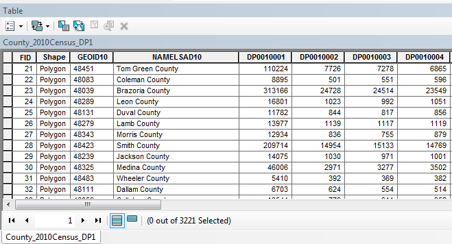
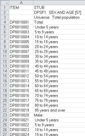
The demographic data columns start at DP0010001 and continue to the right. An Excel table is provided along with each downloaded shapefile, which provides descriptions for each column name. For example, the column “DP0010023” contains the number of males from 10 to 14 years old:
American Community Survey 5-Year Estimates
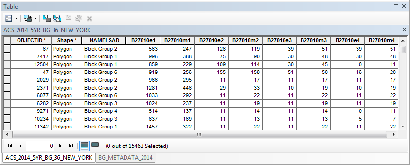
Detailed Tables (2008-2012, 2009-2013, 2010-2014) – Data can be downloaded for several different geographies, but probably the most useful to you will be the Block Group, Census Tract, or County geographies by state. After downloading the data, view the contents of the geodatabase in the ArcCatalog (or the Catalog window in ArcMap) and note that it contains a feature class and several tables. This is a look at the geodatabase I downloaded containing the ACS 2014 5-year estimates (under “Detailed Tables”) at the block group level for New York State:
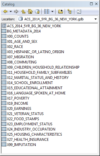
The tables contain the demographic and socioeconomic data, which can be joined to the feature class in ArcMap on the GEOID_Data column in the feature class and the GEOID field in any of the tables. Again, like the Demographic Profile 1 data, you’ll notice that the field names are a little cryptic. A key with descriptions for all the columns is provided in the BG_METADATA_2014 table.
Block Group Data (2006-2010, 2007-2011) – Detailed block group level data provided by state. The data is structured similarly to the Detailed Tables above.
Data Profiles (2006-2010, 2007-2011) – These data sets contain selected social, economic, housing, and demographic characteristics and are available only at the County, Census, and Metropolitan and Micropolitan Statistical Areas geographies.
Mapping the data
You still have to join the tables in the geodatabases provided to the feature class layers, but at least it’s all there for you in one dataset. You don’t have to navigate the American Factfinder, and there’s no table manipulation needed to join the data. Just add the feature class to your ArcMap layout, and then perform the table join.
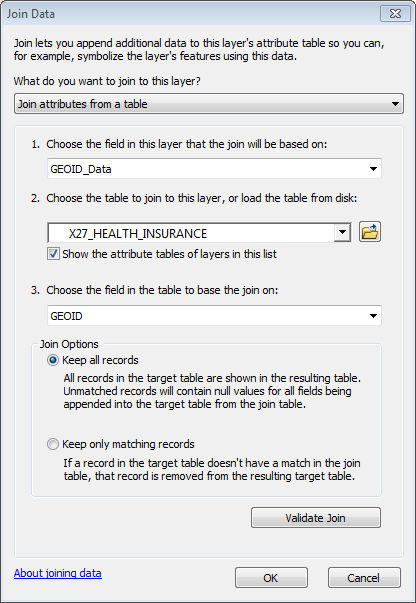
Joining the statistical tables to the feature class
Make sure you join with the GEOID_Data column in the feature class attribute table on the GEOID column in any of the statistical tables. Here, I’m joining the Health Insurance statistics table to the feature class from the geodatabase I downloaded containing the ACS 2014 5-year estimates (under “Detailed Tables”) at the block group level for New York State.
Finding a column to map
With the X27_HEALTH_INSURANCE table joined to the blocks layer, I could then see all the health insurance statistics in the attribute table. Exploring the table, I found that all the column names began with B27010…
A look at the BG_METADATA_2014 table in the geodatabase confirmed that all the statistics in this table are related to health insurance coverage.
Seeing that data included health insurance coverage statistics by age group, I decided I wanted to map the proportion of youth (population < 18 years old) without health insurance. To do so, I had to normalize the data – i.e., divide the number of youth without health insurance (column ‘B27010e17’) by the total number of youth (column ‘B27010e2’). The BG_METADATA_2014 table provides the descriptions for these two fields:
- B27010e17: TYPES OF HEALTH INSURANCE COVERAGE BY AGE: Under 18 years: No health insurance coverage: Civilian noninstitutionalized population — (Estimate)
- B27010e2: TYPES OF HEALTH INSURANCE COVERAGE BY AGE: Under 18 years: Civilian noninstitutionalized population — (Estimate)
If you took Geog/Esci 220: Cartography, recall that when mapping quantities represented by shaded polygons of different sizes, it is appropriate to base the shading on fractions or proportions/percentages of a population rather than total values. There’s two ways to do this:
- Use the Symbology tab in the layer properties to select ‘B27010e17’ as the Value and select ‘B27010e2’ as the Normalization data.
- Add a new column to hold the proportional or percentage values, then populate the column using the Field Calculator.
I chose the second method. So, I created a new floating point decimal field called PercYouthUninsured and used the Field Calculator to calculate the proportion of uninsured youth by dividing the two columns: B27010e17/ B27010e2 (then multiplying the product by 100 so that the proportion of youth without health insurance was expressed as a percentage).
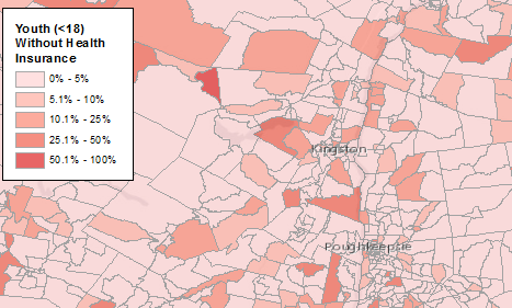
I then used the PercYouthUninsured column to symbolize the quantities. Here’s what it looked like, zoomed in to the mid-Hudson Valley region:
A final note on “margin of error”
It was mentioned earlier in this post that the statistics tabulated in the ACS are estimates based on a sample, not the entire population, and that this method produces some error. Notice in the statistical tables in any of the ACS statistical tables provided in these data sets that the columns are paired – i.e., for each statistic there is an “estimate” of the value for that variable, and a “margin of error” number provided as well.
In the example above, the column B27010e17 is the estimate and the column B27010m17 is the margin of error. (Note the “e” for “estimate” and “m” for “margin of error” in the column name.) The error can be quite large in some cases. For example, in the block group just north of Vassar’s main campus the total estimated youth (<18) without health insurance is 26 and the margin of error is 41. ACS estimates should therefore be taken with a grain of salt… how much of a grain of salt is something I will research and attempt to answer in a subsequent post.