
In this post I will present my actual data findings with minimal interpretation. In the next blog post, “Conclusion,” I will interpret the data I collected and compare it to expected values.
Preliminary Data Recap:
In my previous post I had measured the discharge of several different capacitor values in series with an inductor.
Below were the resulting plots of Voltage vs Time (Figures 1-3):
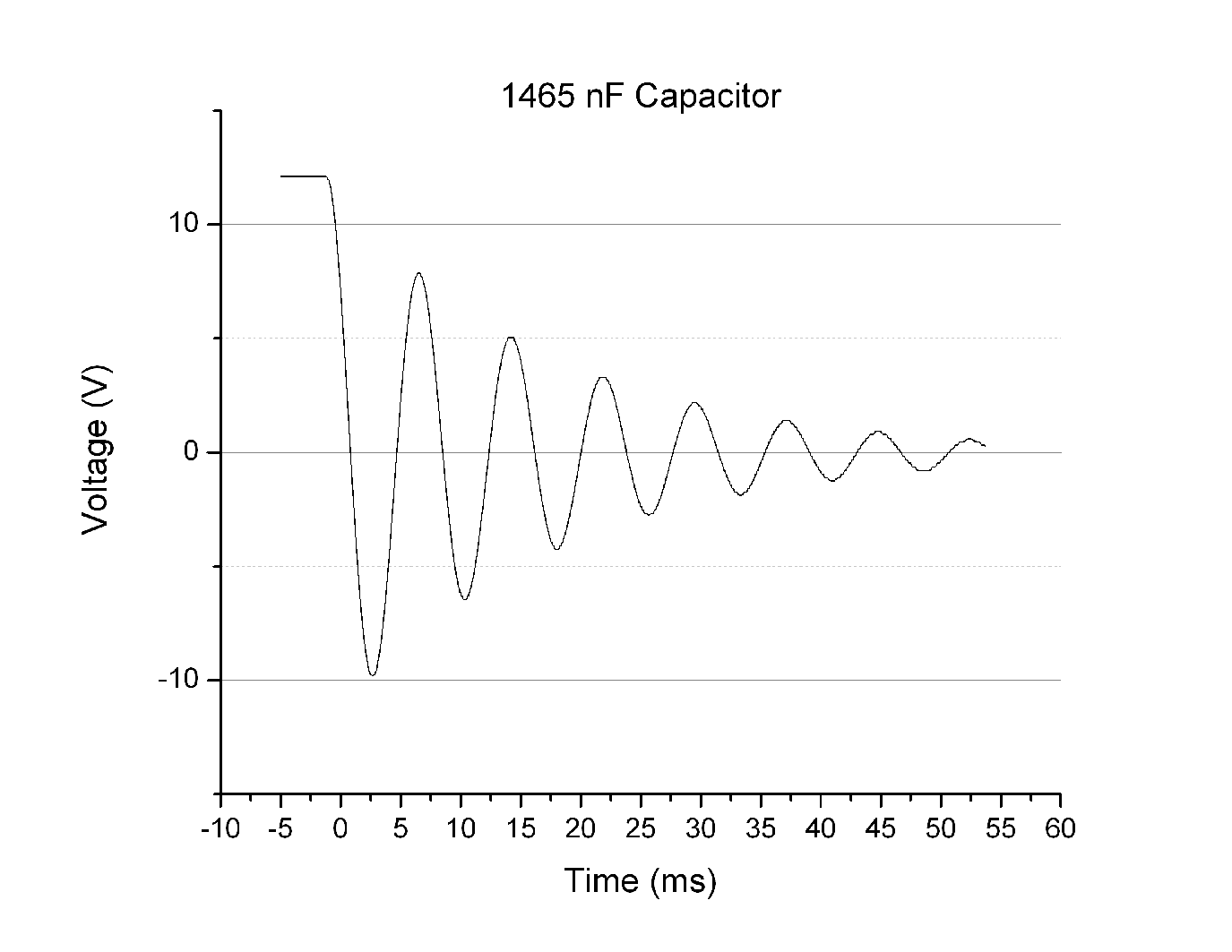
Figure 1
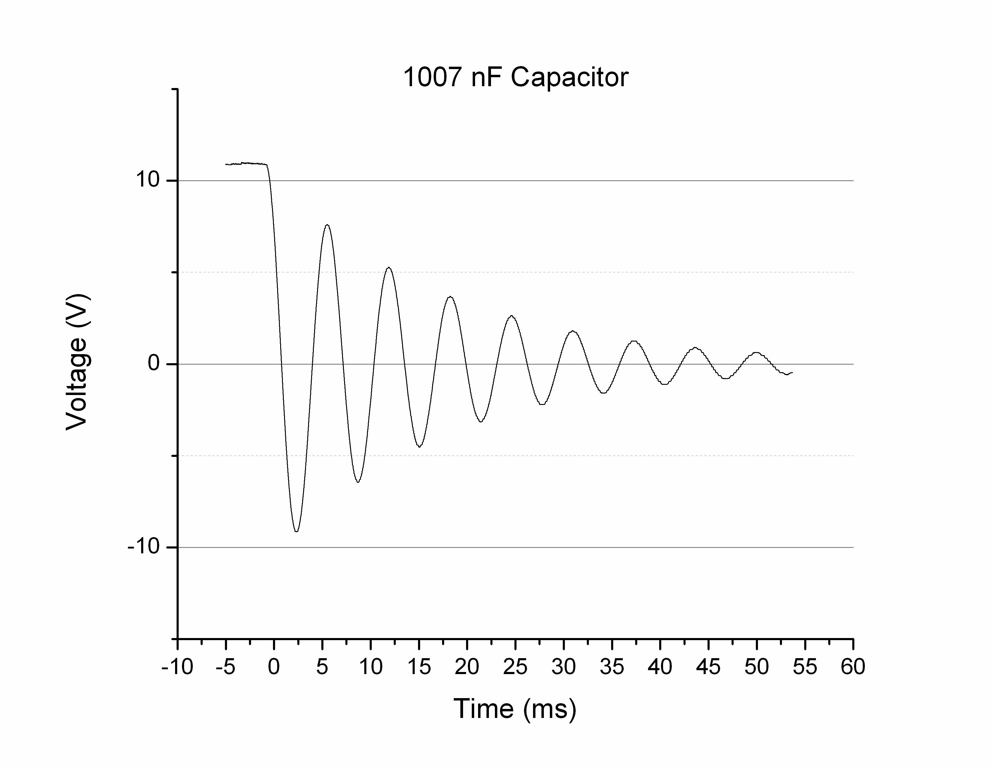
Figure 2

Figure 3
For the 1465, 1007, and 47 nF capacitors the measured frequency of oscillation was 128, 155, and 730 Hz, respectively.
Voltage As a Function Of Time and Frequency of Oscillation
It is helpful to layer these three plots on top of each other (Figure 4). In doing so we can readily compare the curves to each other.

Figure 4
From Figure 4 it is evident that the higher the capacitor value, the lower the frequency of oscillation. This is not surprising, given the equation that the frequency and inductor*capacitor product are inversely related:  .
.
How are frequency and capacitance, or frequency and inductance related? I recorded the frequency of oscillation in several different LC circuits to try and illustrate this relationship. For three different inductor values I discharged five different capacitor values. The resulting plot (Figure 5) is below:
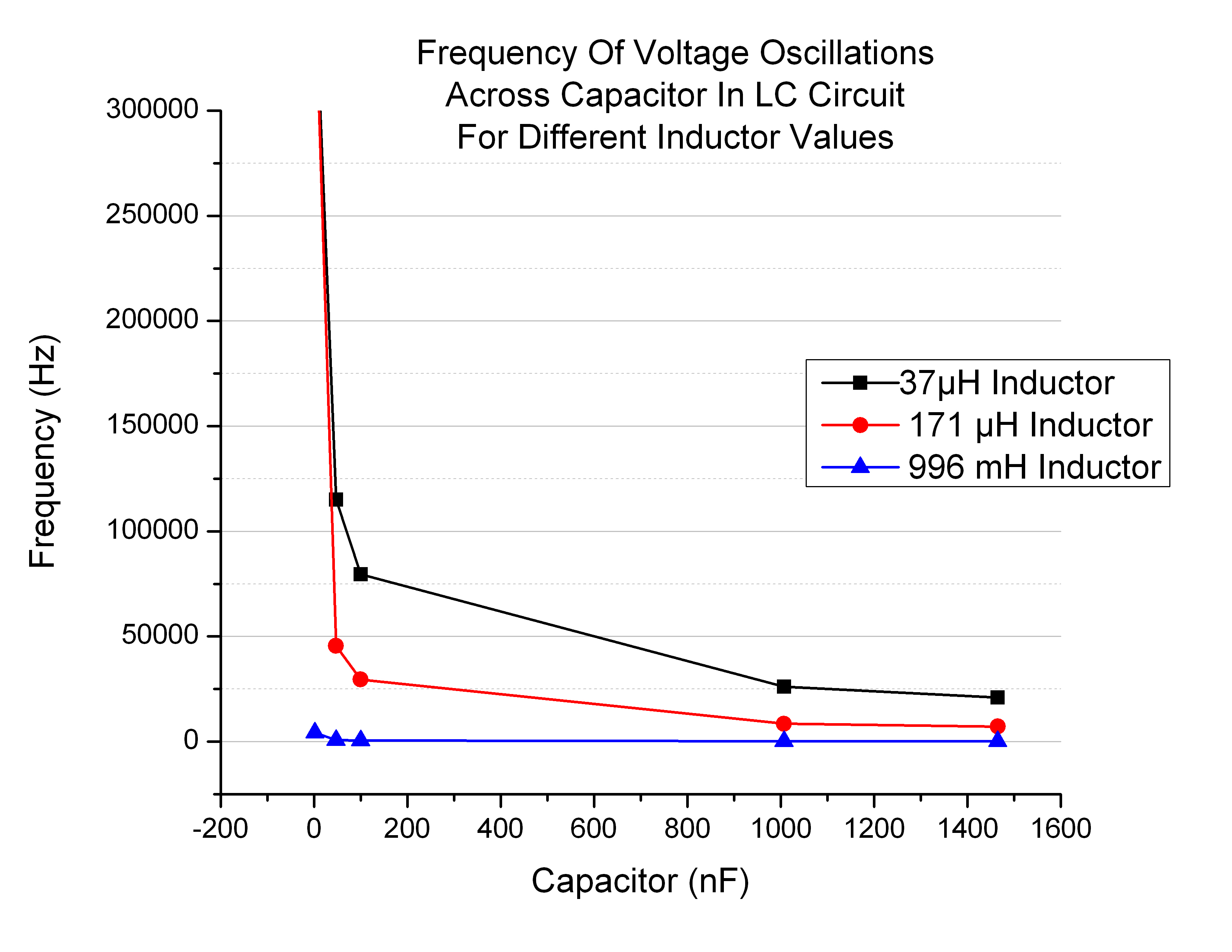
Figure 5
Because it is harder to see the shape of the blue line in Figure 5, I plotted it separately (Figure 6):
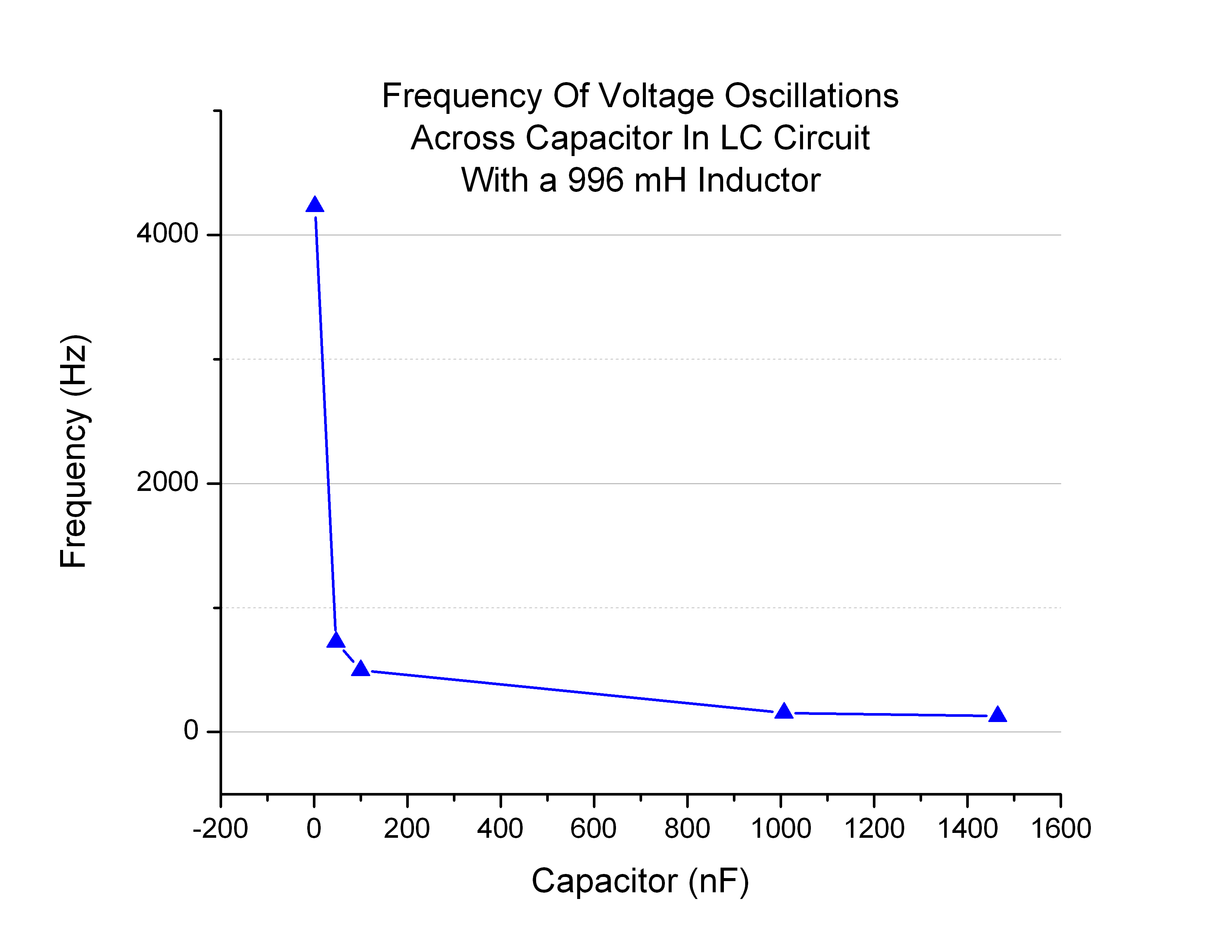
Figure 6
Figures 5 and 6 experimentally illustrate the inverse square root relationship between frequency and capacitance/inductance.
I then plotted the frequency of oscillation with respect to inductor value (Figure 7):
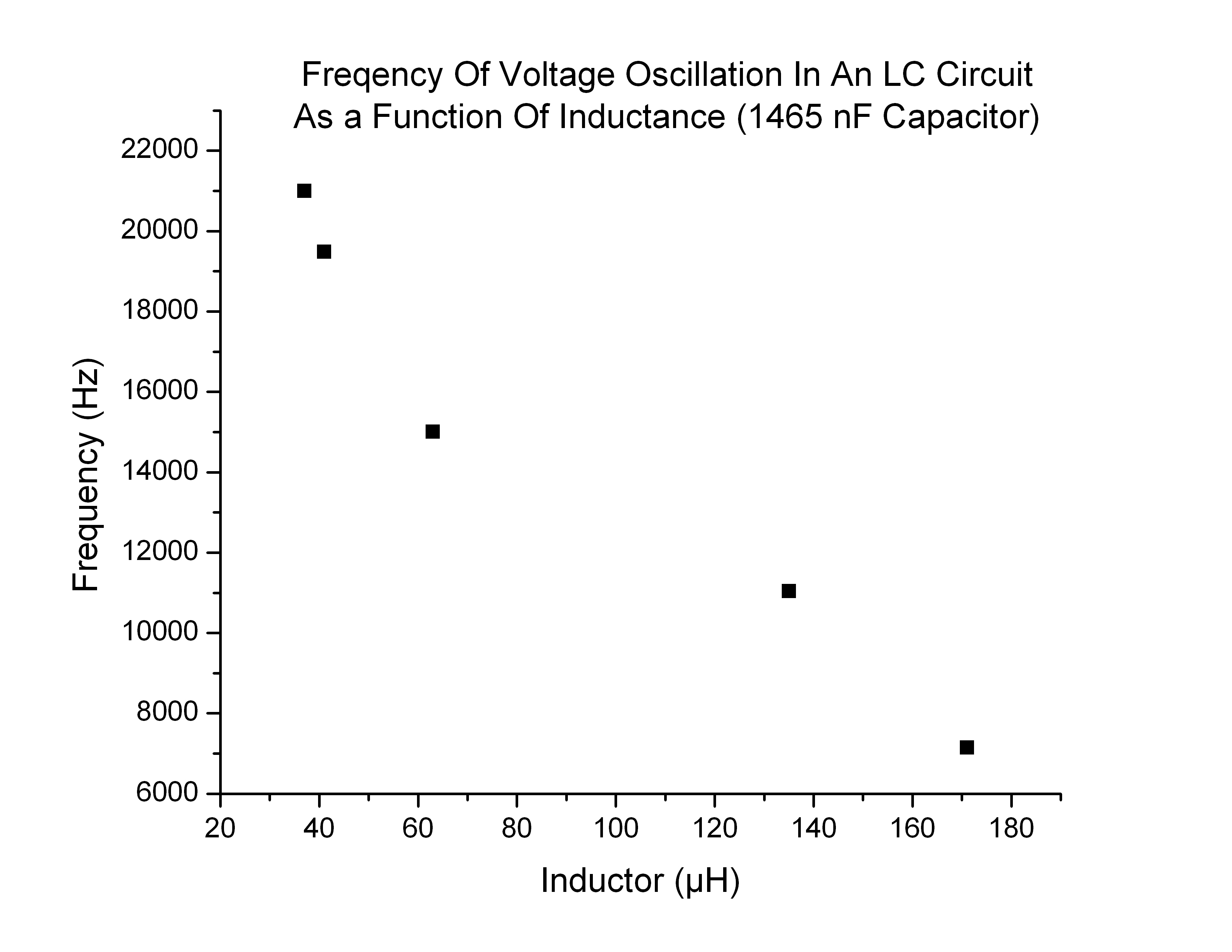
Figure 7
Exponential Rate Of Decay
If you take a look at Figure 4 again, notice that despite changing capacitor values, the exponential decay of each curve is relatively the same. The decay for each curve is the same because the decay coefficient β is a function of resistance and inductance, not capacitance( ). In Equation (1) you can see the decay term of the voltage, e^(-βt):
 (1)
(1)
In order to measure the decay constant I used Origin Pro to fit an exponential curve to the peaks of the voltage plots. The formula used for this function fit was as follows:
Where R0 is the decay coefficient, -β
Figure 8 below is an example of this function fit:
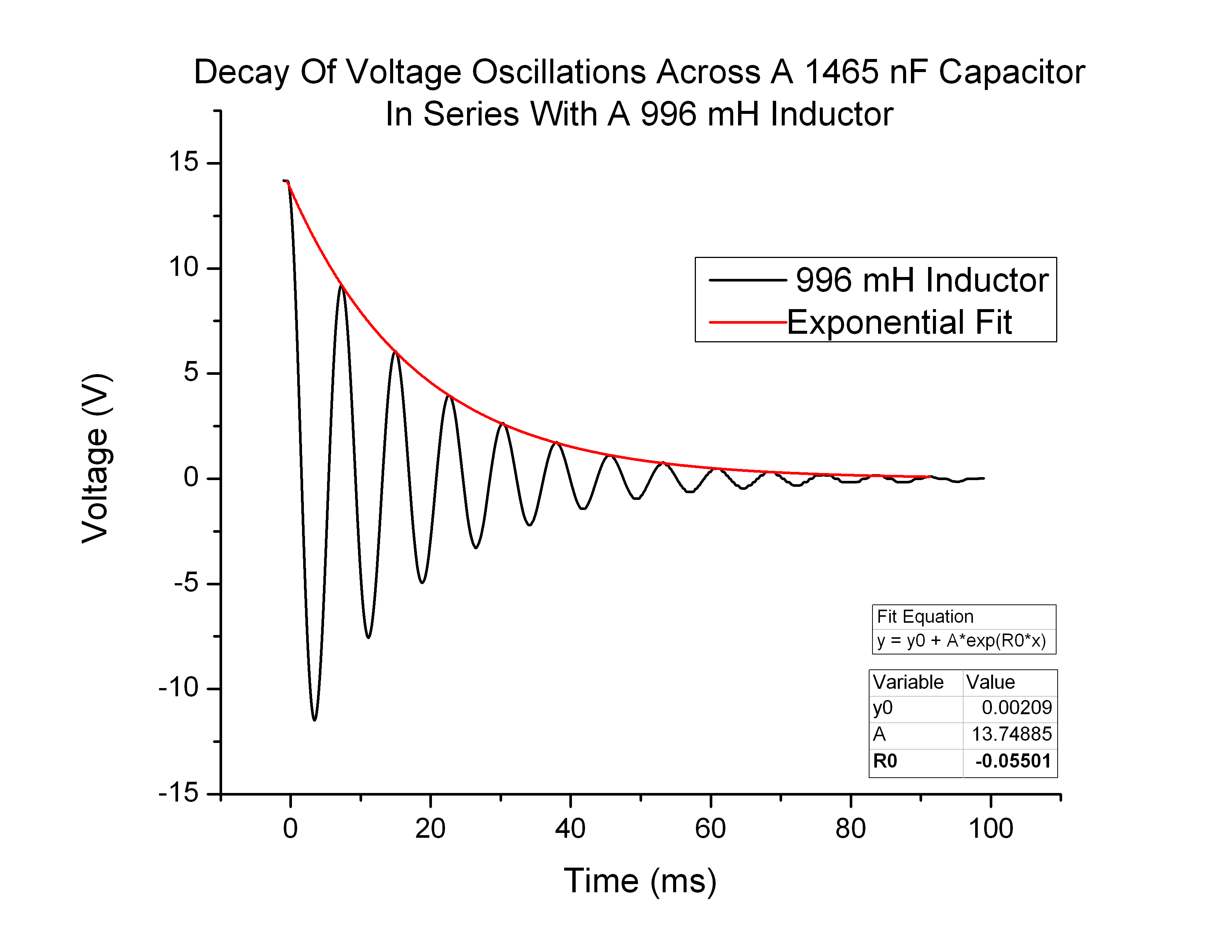
Figure 8
I fit an exponential function to the 996 mH and 1007 nF, 47 nF oscillations as well, resulting in the table below (Figure 9):
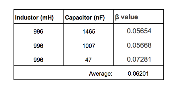
Figure 9
Theoretically the β value should be the same for all of them.
In order to explore how the decay coefficient β changes I needed to change the inductor values. Because the voltage curves were more manageable at greater LC values, I used the largest capacitor I had and varied the inductor value. The results were as follows (Figures 10-11):
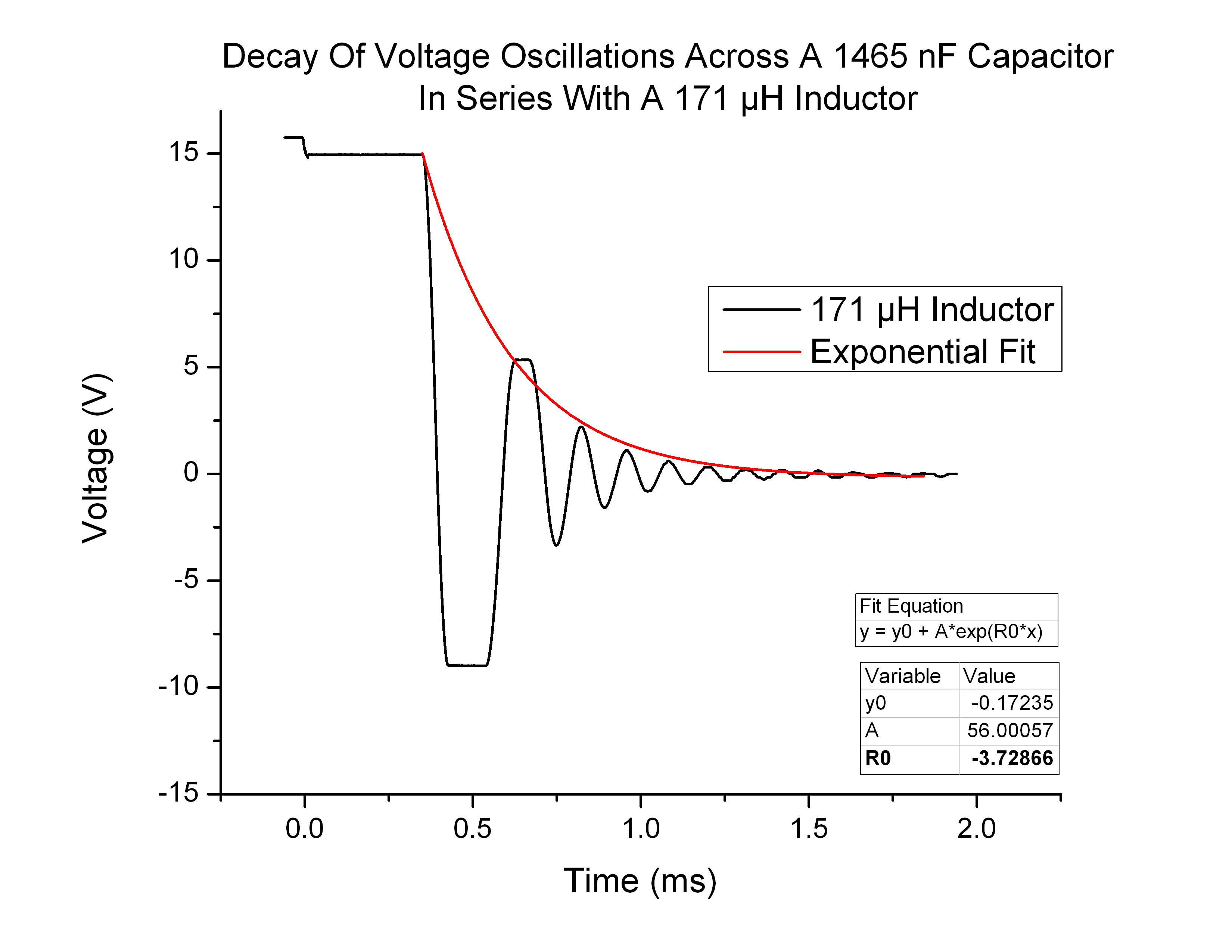
Figure 10
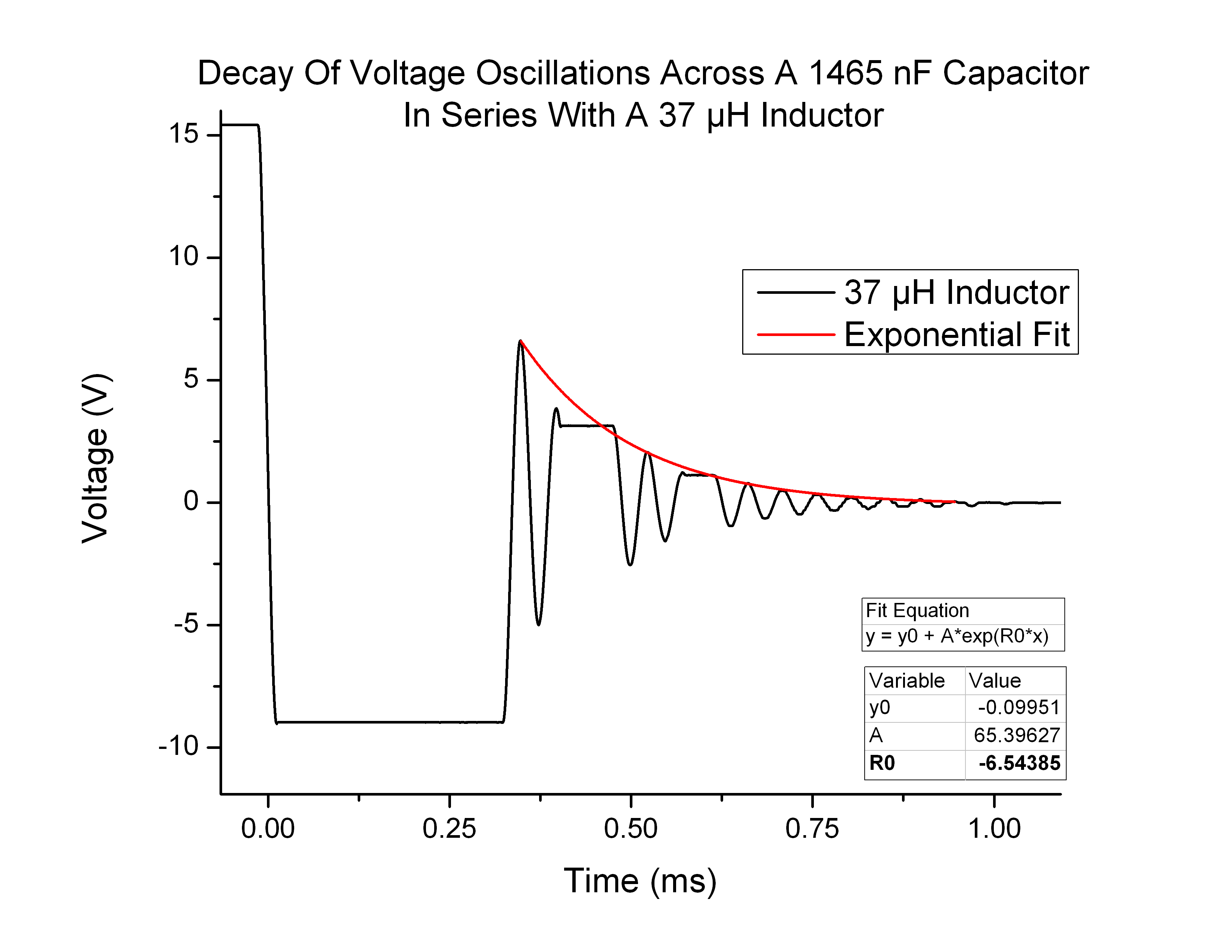
Figure 11
The resulting decay coefficients are as follows (Figure 12):
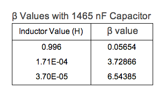
Figure 12
Which can also be represented in as a scatter plot, despite having so few points(Figure 13):
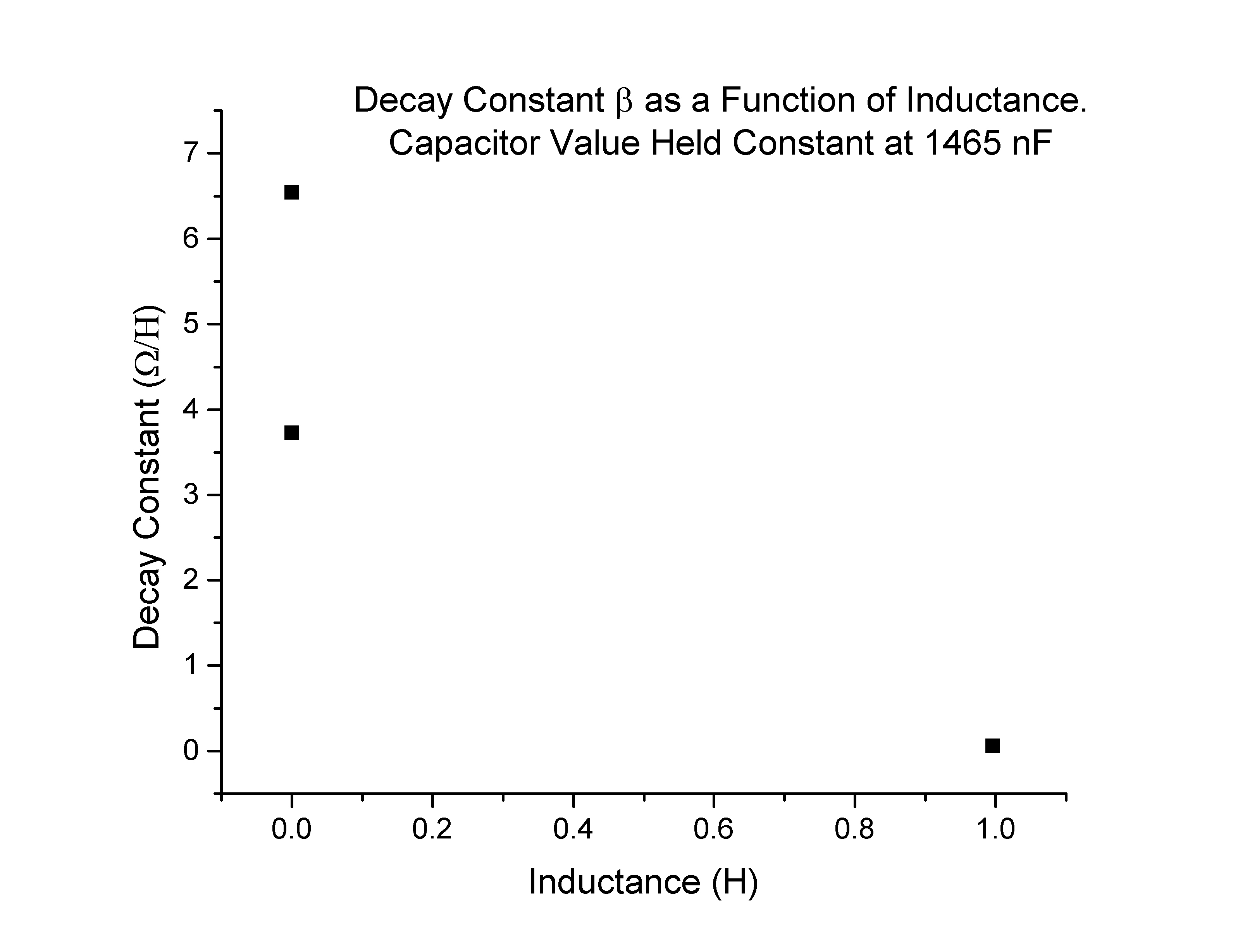
Figure 13
