Category Archives: Theo

Conclusion/Overview

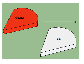
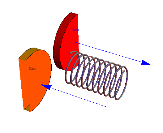
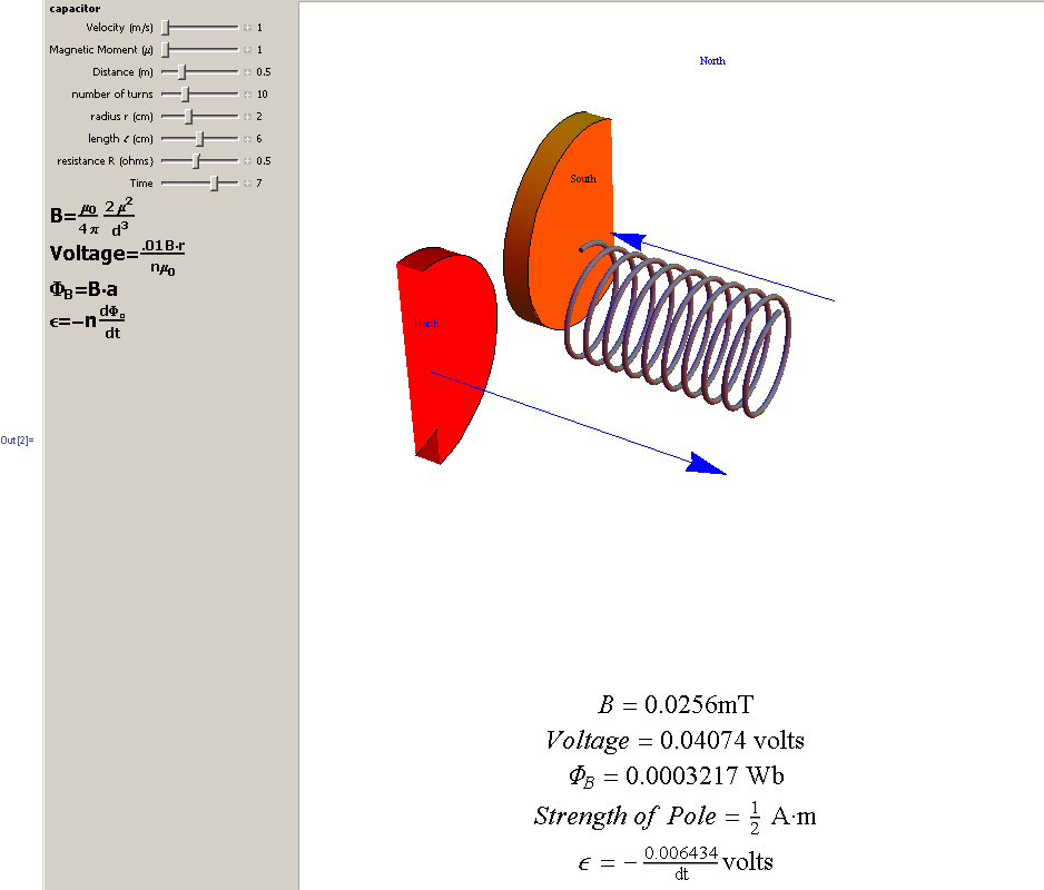
Mistakes were made throughout this process. Some were as simple as a dropped variable and others were intensely more complicated. In the end I was still able to produce what I set out to do: An interactive animation that allows you to see how a single coil in a stator of magnetic induction based wind turbine creates current.

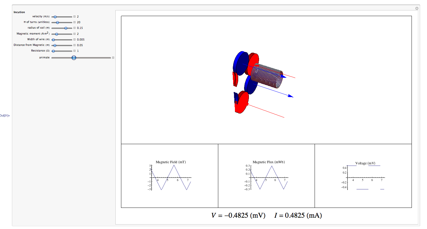
Much of the work I did was simply writing the code to get the interactive animation to function properly. Below is a screenshot, but the important code is linked to at the end of this post.

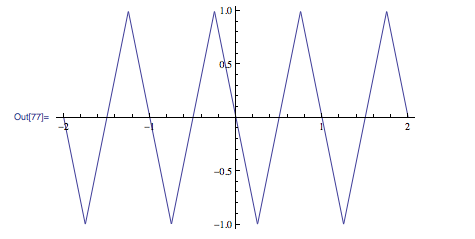
Just to recap some of the derivation I did in earlier posts, I will present a short breakdown here. I started with the basic equation for B, but in order to have the magnetic field change over time based on my magnet array, I had to use a triangle wave. In my previous post I inserted values for the period, but in my Mathematica code, I made it dependent on the velocity so that all the graphs would match up.

Triangle Wave Function:

(1)   \begin{equation*} \frac{4}{d/v}\left [ (t-2d/v)\cdot \left \lfloor \frac{2td}{v}+.5 \right \rfloor \right ]\cdot (-1)^{\left \lfloor \frac{2td}{v}+.5 \right \rfloor} \end{equation*}

Magnetic Field Equation

(2)   \begin{equation*} B=\frac{2\mu }{d^{3}}10^{-4}\frac{4}{d/v}\left [ (t-2d/v)\cdot \left \lfloor \frac{2td}{v}+.5 \right \rfloor \right ]\cdot (-1)^{\left \lfloor \frac{2td}{v}+.5 \right \rfloor} \end{equation*}

Once I had my B(t) I quickly found the flux, but to get to the voltage I had to find the derivative of my triangle wave based B(t) function. I made a square wave approximation to solve for the derivative. In my last post I again plugged in constants in order to show the look of the graph, but in my code I made it dependent on all of the variables.

(3)   \begin{equation*} \frac{4\pi \mu d_{w}rN}{d^{3}}\cdot \frac{4}{d/v}10^{-4}\cdot (-1)^{\left \lfloor \frac{2td}{v}+.5 \right \rfloor} \end{equation*}

Using this square wave approximation I was able to find the voltage in the coil. Once I had a formula for the voltage, the induced current was simple to find.

At this point I noticed a grave mistake with my approach to this problem. By approximating the magnetic field with a triangle wave, I made it so the voltage simply flipped back and forth from negative to positive with no gradation. In hindsight it would have been better to use a version of a sin wave as an approximation. That would present its own issues, as the magnetic field would have a fairly linear change. With more time I would have attempted to find a better approximation for the magnetic field that was easier to use.

It should also be noted that my last post had a few typos in it that could be very confusing. I wrote the equation:

(4)   \begin{equation*} B=\frac{\mu _{0}}{4\Pi }\frac{2\mu^{3}}{d^{3}} \end{equation*}

but it should read:

(5)   \begin{equation*} B=\frac{\mu _{0}}{4\pi }\frac{2\mu}{d^{3}} \end{equation*}

The mu was confused for most of the post, but I was able to correct the issues I had with it for all of the formulas in this post and the code.

Code: https://vspace.vassar.edu/thvandermeer/Trying%20to%20get%20graphs%20in%20it.nb

Share

As discussed before, I will be looking at how magnetic fields induce currents in wire coils. The setup I have chosen to focus on has magnets passing over a stationary coil as shown below.

For the purpose of my diagram, we see a north, a south, and another north pass over the coil. Each magnet has a radius of 2cm and 1cm gap between them. This is one of the few things that is not variable in my animation.

The first thing I will concern myself with is producing the equation for the magnetic field. I will start with the following equation:

(1)   \begin{equation*} B=\frac{\mu _{0}}{4\Pi }\frac{2\mu^{3}}{d^{3}} \end{equation*}

After plugging in the constant for \mu_{0} and scaling it to get millitesla I get the equation:

(2)   \begin{equation*} B=\frac{2\mu^{3}}{d^{3}}*10^{-4}\;\;\;mT \end{equation*}

Aha! I have the magnetic field dependent on distance. This is great, but I am more interested in having one dependent on time. Here is where the heavy lifting comes in. I will now assume that all of my other variables are constant, with the exception of time. Time should only effect one thing with the magnetic field, and that is the direction of the field. This changing magnetic field is the exact effect that we need to make induction work. Since the only change is the direction we know that the range of the field is -B to B. This means that we need a function that oscillates linearly from 1 to -1 and then multiply our equation derived for B by this new oscillating function.

The reason I chose a linear function, is because as one magnet moves away an opposite one moves in. I am going to make the assumption that when the north facing and south facing magnets are equidistant from the center of the coil, the magnet field within is zero. What I hope to achieve is a function that will linearly rise and fall from 1 to -1, and what better way to do that than with a triangle function.

The equation for this triangle function is:

(3)   \begin{equation*} \frac{4}{p}\left ( \left ( t+.5 \right ) -\frac{p}{2}\left \lfloor \frac{(2t+1)}{p}+.5 \right \rfloor\right )\cdot (-1)^{\left \lfloor \frac{(2t+1)}{p}+.5 \right \rfloor} \end{equation*}

Where p is the period, and the bottom side brackets \left \lfloor floor \;fn \right \rfloor are floor functions.

As stated earlier the magnets have a radius of 2cm and separation distance of 1cm. Since this is constant we know that the distance between the peaks of the triangle function has to be 10cm (2+1+4+1+2) using the equation v=\frac{d}{t} we can say that p=\frac{.1m}{v}.

Using this new definition of p, (and assuming v is constant) we get the following equation:

(4)   \begin{equation*} 40v\left ( \left ( t+.5 \right ) -\frac{.05}{v}\left \lfloor \frac{(2t+1)v}{.1}+.5 \right \rfloor\right )\cdot (-1)^{\left \lfloor \frac{(2t+1)v}{.1}+.5 \right \rfloor} \end{equation*}

which in turn leads us directly into our new equation for B:

(5)   \begin{equation*} B(t)=\frac{2\mu^{3}}{d^{3}}10^{-4}\cdot40v\left ( \left ( t+.5 \right ) -\frac{.05}{v}\left \lfloor \frac{(2t+1)v}{.1}+.5 \right \rfloor\right )\cdot (-1)^{\left \lfloor \frac{(2t+1)v}{.1}+.5 \right \rfloor} \end{equation*}

We have successfully found B as a function of t!

Now we have the magnetic field some distance from the magnet. The next step is to find the flux. Since in my diagram the magnet is larger than the coil (and at most the same size) I will only worry about the coil’s area. I also have no pitch on the magnets or wire, so angle is irrelevant and will be ignored from here on. Using the following equation:

(6)   \begin{equation*} \Phi _{B}=\int B\cdot da \end{equation*}

we find:

(7)   \begin{equation*} \Phi _{B}=\frac{2\mu^{3}}{d^{3}}10^{-4}\pi r^{2}d_{w}N=Nd_{w}\frac{2\pi r^{2} \mu^{2}}{d^{3}}10^{-4} \;mW \end{equation*}

Where d_{w} is the diameter of the wire and N is the number of turns.

Since one of the main goals is to find the emf, we need to find \Phi_{B} with respect to t. Luckily, we did most of the work already when we derived B(t). The new equation reads:

(8)   \begin{equation*} Nd_{w}\frac{2\pi r^{2} \mu^{2}}{d^{3}}10^{-4}40v\left ( \left ( t+.5 \right ) -\frac{.05}{v}\left \lfloor \frac{(2t+1)v}{.1}+.5 \right \rfloor\right )\cdot (-1)^{\left \lfloor \frac{(2t+1)v}{.1}+.5 \right \rfloor} \;mW \end{equation*}

For simplicity I will quickly denote C=-Nd_{w}\frac{2\pi r^{2} \mu^{2}}{d^{3}}10^{-4}40v

We can now move along to the emf!

(9)   \begin{equation*} \varepsilon = -\frac{d\Phi_{B}}{dt} \end{equation*}

Plugging in our absurdly long equation for the flux, we get:

(10)   \begin{equation*} \varepsilon = C\frac{d\left ( \left ( t+.5 \right ) -\frac{.05}{v}\left \lfloor \frac{(2t+1)v}{.1}+.5 \right \rfloor\right )\cdot (-1)^{\left \lfloor \frac{(2t+1)v}{.1}+.5 \right \rfloor}}{dt} \end{equation*}

How would you take a derivative of this triangle function with respect to t? Well, you can’t. At least, I can’t, but what I can do is find an adequate approximation. I know that the positive slope is .025v^{-1} and the negative slope is -.025v^{-1}. From here I can ascertain the derivative simply by finding a function that flips back and forth between those two values every .05v^{-1}, which should look like a square function.
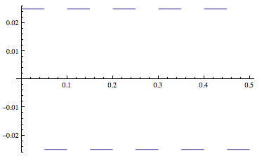
The equation for which is:

(11)   \begin{equation*} .025\cdot sgn [sin(\frac{\pi t}{.05v)}] \end{equation*}

Where the sgn function simply takes all positive values and makes them 1 and all negative values and makes them -1. This gives us an emf of:

(12)   \begin{equation*} \varepsilon = C \cdot .025\cdot sgn [sin(\frac{\pi t}{.05v})] \end{equation*}

and an induced current of

(13)   \begin{equation*} I(t)=\frac{\varepsilon}{R}=.025C \frac {sgn [sin(\frac{\pi t}{.05v})]}{R} \end{equation*}

HUZZAH!!

Share

Project Proposal 2

For my project I will attempt to model the magnetic field from a magnet as it interacts with a wire coil. I will make an interactive model that can vary speed, distance of coil to magnet, magnet intensity, and number of turns among other things. My first attempt at the animation can be seen below.

And here it is to illustrate the movement:


As is evident by this picture, I still have yet to add the magnetic field lines, and that is where the bulk of my project will be. I will be using our Griffiths textbook, The Art of Electronics by Horowitz & Hill, The Handbook of Tables for Applied Engineering Science, and Engineering Circuit Analysis by Hayt and Kemmerly. I also have collected a few journal volumes that I will use as I see which are the most useful.

I will be using the equation

(1)   \begin{equation*} B=\frac{\mu _{0}2\mu^{2}}{4\Pi d^{3}} \end{equation*}

as well as

(2)   \begin{equation*} \Phi ^{_{B}}=Ba \end{equation*}

   and  

(3)   \begin{equation*}     \epsilon =-n\frac{d\Phi _{B}}{dt}   \end{equation*}

Where \mu is the Magnetic Moment, \epsilon is the electromotive force, and \Phi^{_{B}}

Since I will have the magnet moving over a stationary wire coil, we will see that electric fields (not magnetic forces) are responsible for setting up the emf. Although the electric and magnetic fields are inextricable linked, it is useful to note that because stationary charges can’t experience magnetic forces, there has to be another explanation.


The unanswered question is how to mathematically model the magnetic field due to these magnets. I currently will be simplifying each magnet to a magnetic dipole, as opposed to a more complex magnet.  I would hope to have their intensities change as I change the magnetic moment, and I would also like to see what kind of feedback the solenoid would produce. In order to simplify this process the next iteration of my animation will be a square magnet and a square coil. This should hopefully make the modeling easier, as their seems to be more information on that kind of a set-up.


Share

Proposal

For my project I will be investigating electromagnetic induction in wind turbines. I will attempt to flesh out the equations related to efficiencies. I will specifically look at how turns of wire coils and surface area of the blades pertain to energy output. Magnetic induction generators output AC current, and I will try to have my analysis reach through the entire process up until this point. I will use equations such as:

Using information from The Handbook of Tables for Applied Engineering Science I will explain and attempt to animate equations such as L=FN2d. This equation helps with showing how solenoids proprieties affect the inductance. If time and ability permit, I will also look try and present an animation explaining the phase shifts in stator wire arrays. I will specifically look into the magnet wire construction as shown in the figure below.


With this type of arrangement we will see that electric fields (not magnetic forces) are responsible for setting up the emf. Although the electric and magnetic fields are inextricable linked, it is useful to note that because stationary charges can’t experience magnetic forces, there has to be another explanation. In my project I will try and present this subtle discrepancy through animations. Much of the information I will collect will come from chapter seven of Griffiths, and various journals, as well as the book mentioned above and The Art of Electronics.

Share

Theo

Magnetic induction is the main component of energy production in wind turbines. The efficiency of this energy production is based on wire turns and the power of the magnets used. To examine this more closely I will attempt to model the efficiencies of different arrangements. I hope to look at both different magnets, and different wire arrangements in order to flesh out how efficient magnetic induction based turbines are. Chapter seven of Griffiths touches on the subject, but does not delve into its real world applications as much as I hope to.

Share