For this first week, Magnes instructed me to just write a summary of last semester. During the second week, I worked on setting everything I worked on last semester back up. This included rewiring Arduino circuits and testing the code. I took pictures of the setup and of some of the code for my summary. All of a sudden, the Arduino graphing code stopped working. I spent the rest of the week trying to debug the code. I also met with Lily Frye, the new lab intern, and got her caught up to speed. I explained what we have been doing, where we are in the project, and the type of things she could help out with. I gave her the Arduino project book Bryan and I used last year to learn how to use the device so she could get started. Overall, it was a good week. It’s nice to get back in the swing of things.
Category: Uncategorized
Summary of Research from Last Semester
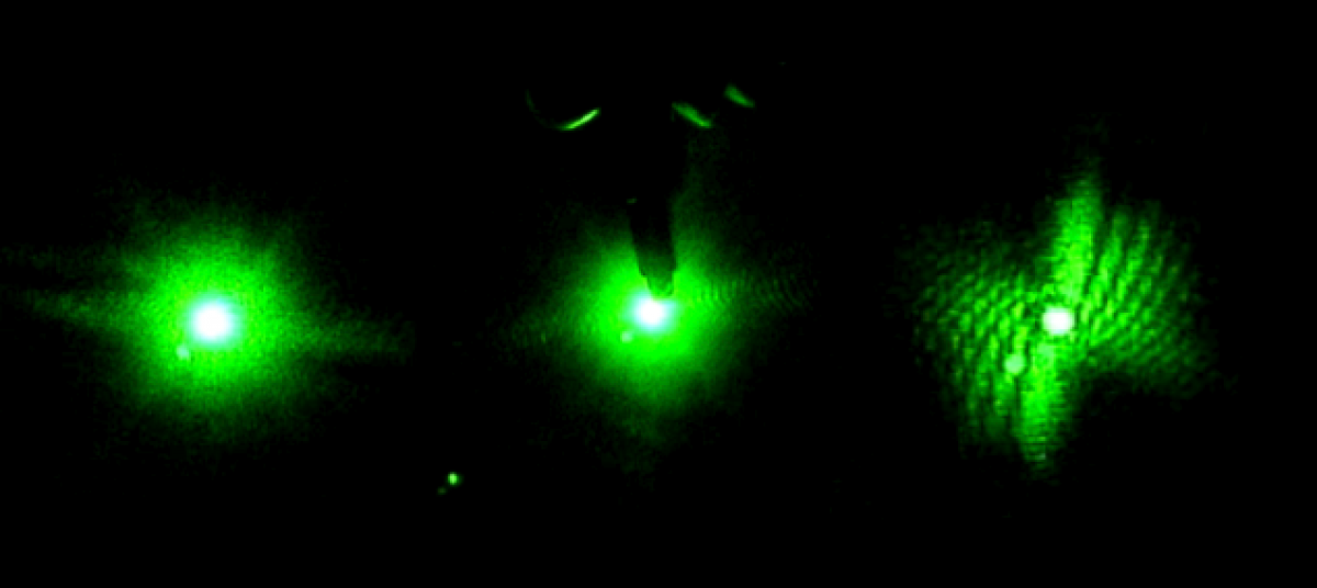
The first week in the lab mostly just involved getting acquainted with the equipment since no worms were available. I watched a laser safety video online so I could properly handle the lasers. They are all fairly safe, although goggles should be worn when using the blue laser to protect against eye damage. Goggles are not needed when handling the Helium-Neon red laser. The table was already set-up by the time I joined the team, but Bryan explained the arrangement to me. A pinhole, beam-splitter, mirrors, optical chopper, and slide holder are used. The table was setup so either laser could be used without having to move it each time. Bryan told me get acquainted with the lasers and Picoscope software by placing small objects, such as strands of hair, in a slide and shining the laser through it. He also showed me how to use the Picoscope software to record data. I practiced this a few times. I also researched the project we were working on by reading about diffraction patterns, Professor Magnes’ research, and by reading the project blog.
Later on, I got to work with live worms. Bryan showed me how to take one from a petri dish using a microscope, suspend it in a cuvette filled with water, and record data by shining the laser light through it. It was sometimes surprisingly challenging to catch a worm, but also kind of fun. I quickly learned how to keep the worm in the laser light. If it moved out of the light, the Picoscope graph would flat line. The Picoscope graphs the voltage induced by the diffracted light hitting a photosensor.
Soon after, Bryan told me about a side project Professor Magnes asked him to work on. When I showed interest, he asked if I wanted to work on it with him. Our goal is to program an Arduino to collect the diffraction pattern data caused by the C. Ellegans movement and output the thrashing frequency. We started by buying an Arduino starter kit, which came with a lot of useful supplies including resistors, breadboards, an Arduino, buttons, and a project book. I worked with Arduinos a little during the first semester of my senior year of high school, so I was excited to use them again. We started by reading the project book and trying projects to become acquainted with the Arduino and learn how to use it. I began with the basics: setting up an LED and getting it to blink, which was very easy. I then moved on to more complex projects. Bryan created a “crystal ball” that wrote yes/no responses on an LCD when the Arduino was tilted. He was having trouble getting it to work, but I managed to find a problem with how he wired it.
He thought LCD screens might come in handy, so I did a little research on how to program and use them. I found a light meter project online, which measured the levels of light in the room using a photosensor and displayed the percent brightness on an LCD screen. It seemed like it might teach me skills that could be useful for the project so I decided to build it. However, the code used functions that were not compatible with the Arduino and LCD I was using. Nonetheless, it provided a useful, general outline to work from. I was able to write my own code and use my newfound LCD knowledge to program the light sensor.
Next I moved on to learning to output graphs with the Arduino, another potentially useful tool. I used Processing, an open source programming language and development environment that is compatible with Arduinos. I found instructions for graphing Arduino serial monitor data using Processing on the Arduino site, and successfully graphed data collected from the light sensor in real time. However, I was not satisfied with the graph because it had no axes or scale. I found a more complex graphing code online, and got it to work. I edited the code to have more informative y-axes, which represented voltage, and added x-axes for time.
For some reason, the newer photosensor was not working properly with the Arduino. Bryan gave me the task of trying to fix it. I hooked the photosensor up to analog pin 0 on the Arduino, and sent the data it received to the serial monitor. Then I shone the laser light through the optical chopper and observed the values in the serial monitor. I noticed that it actually was working, but was producing only a very small change in voltage. When I graphed this, it showed a standard square graph, as expected. I messed around with the Arduino code trying to make the voltage difference larger, but I was not convinced that was the right solution. This would not improve the connection between the Arduino and photosensor or give more accurate results. I did not make much more progress on this front since I ran out of time, although it did seem to be working fairly well. I did some testing to see how accurate it was. At very high frequencies, the Arduino and graphing code had some trouble keeping up, but for our purposes it should work fine.
Bryan’s initial idea for the Arduino project was to use Fourier transforms. However, we quickly moved on to RLC circuits. I researched both of these concepts since I was unfamiliar with them. Bryan was having trouble successfully making an RLC circuit and spoke with someone in the Physics department about it. Apparently, RLC circuits are great in theory, but a little difficult to get to work in reality. We were unable to solve this problem last semester. I did a little research over the break, and my current idea is to either buy or build a band-pass filter. I could not find one online that allowed low enough frequencies through, but plan on searching more in depth when I get back to the laboratory next week. If that fails, I found an Instructables post about making one that looked promising, and I will attempt to make one myself.
Link to instructables post: http://www.instructables.com/id/Active-Band-Pass-Filters/?ALLSTEPS
Weeks 8 & 9
Two very successful weeks in the lab.
We have continued running data on the worms with the blue laser. We changed the scale on the x axis of the picoscope software to collect data in intervals of 10 seconds per frame instead of 1 second per frame. This is the match the data from over the summer. Sadly, we found out that we have been collecting data with the intensity of the laser at too high of a value. Mostly we had been using the laser at a power of about 5mW. Over the summer they ran data with the laser at a power of around 1.5mW. In order to add to the data from over the summer, we must have the same power. Therefore all the trials we ran with 5mW, will not be useful for this data analysis. Hopefully we can find a use for those data sets.
We had to realign the laser some because it happened to somehow be out of alignment. Later in week nine we realized that the picoscope was reading a very low value for the power of the laser. We think it was due to the fact that Brian turned all the photo diodes off one day.
This brings us to the end of the semester. After a bit of a slow start, in order to get accumulated with the lab, I think we had a very successful semester. We came to a realization that we cannot get that much work done in the lab during the semester due to the sheer lack of time. Over the summer, approximately 40 hours a week are spent working in the lab, while we only spent 3.5 hours a week in the lab this semester. I look forward to continuing research next semester, and hopefully starting some data analysis to find out what our data is really telling us!
Weeks 5-7
I have been extremely busy as of lately, and apologize for not posting earlier.
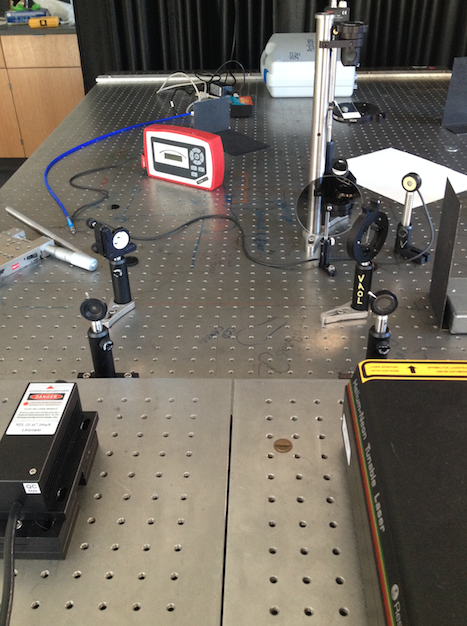
Week 5 was shortened due to fall break. Therefore we only were able to work in the lab one day. We finished the setup and alignment for the blue laser that day. Below is a picture of the blue laser final set up. It is very similar to the previous table set up, however we got rid of the beam splitter.
Week 6 saw a slight set back in the lab. Over break, due to miscommunication between Brian and Elias, our worm stock was never harvested. We came back from break to an empty incubator. All our previous stocks had been discarded! We began a new stock, but had to wait until later in the week to collect any data on the worms.
Week 7 was a very productive week in the lab. Eli and I developed a good system to collect data with using the blue laser. Wearing the safety goggles makes it more difficult to view the worm and also the laser beam itself. One of us starts the PicoScope software, and then quickly walks over and helps the other find the worm and get the diode positioned so the diffraction pattern can be seen.
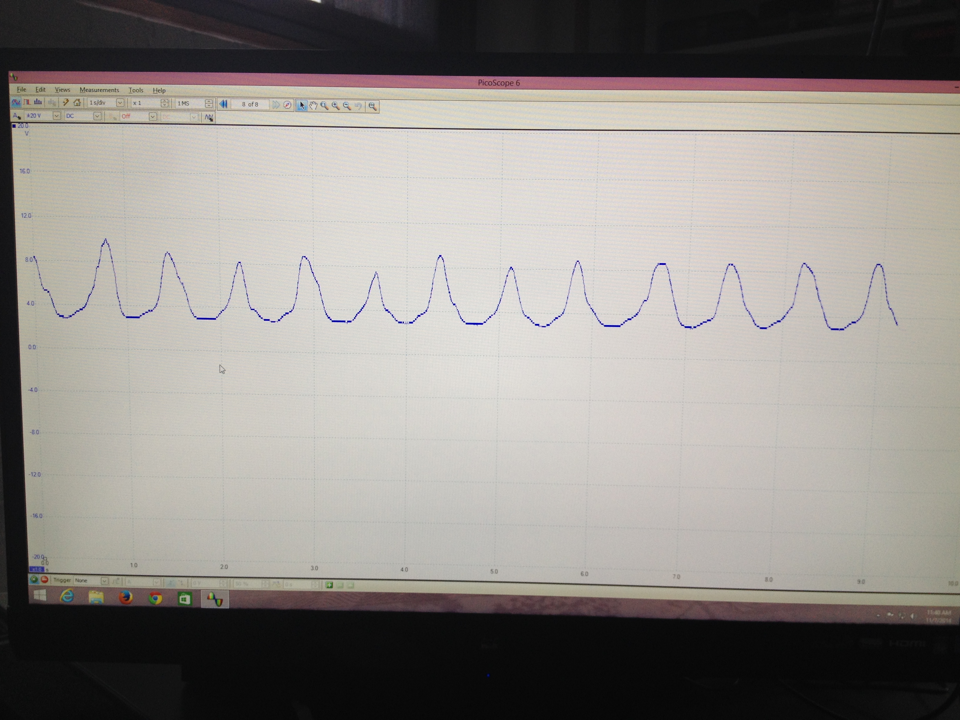
Below is a picture of what the PicoScope data looks like when we collect it. The sinusoidal peaks are the data we are trying to achieve. As the worm moves around in the laser light it changes the diffraction pattern that turns out on the screen as peaks in the graph. We can then use those peaks to analyze to motion of the worms. The flatline sections (none pictured below) in the data are when the worm is not being illuminated by the laser and therefore creates change in the diffraction pattern.
Week 4
Another successful week in the lab.
Early in the week we ran data on the worms with the red laser. With a more efficient procedure, a little more experience under our belts, and an extra set of hands in the lab, we were able to run data and collect data on seven worms in one lab session.
Later in the week we attempting to collect data with the blue laser. However we ran into trouble with the table setup. When we originally set up the table, we used a beam splitter to send both lasers to one slider holder. Using a beam splitter caused the power of the blue laser to be reduced greatly. When we went to use the blue laser to analyze the worms, we could not even see the beam inside the cuvette due to the lack of power and the safety goggles. The laser is too strong to be viewed with the naked eye, and the safety goggles that must be worm make it extremely difficult to view the weak beam.
We began to fix the table set up so that each laser has its own slide holder, and there will be no use of a beam splitter anymore. The new setup is almost finished, we just have to finish aligning the lasers.
Week 3
Exciting things happened this week in the VAOL lab. For the first time this semester we were able to collect data on the worms.
In the beginning of the week we spent time practicing transferring the worms from the cup they are grown in, into a cuvette filled with distilled water. This is more challenging than one would expect because the worms are microscopic and the process must be down under a microscope, using a tiny pick to lift the worms up and transfer them to the cuvette. We also practiced finding the worm once it was in the cuvette and getting the laser to pass through them to create a diffraction pattern. Once the worm is found in the cuvette with the naked eye it is pretty easy to keep the laser on it as it swims around.
Later in the week, we actually collected data using the pico scope software on the computer. The pico scope evaluates the change in diffraction pattern observed by the photo diode as the laser passes through the worms. It then shows the results in voltage. We ran trials on four worms total, getting data for each one using only the red laser. The plan is to continue running data on more worms with both the blue and red lasers, after which we will combine all the data for analysis.
Things are finally starting to come together in the lab after what seemed like a lot of grunt work putting the lab together after the move.
Week 2
This week saw a lot of progress for the lab.
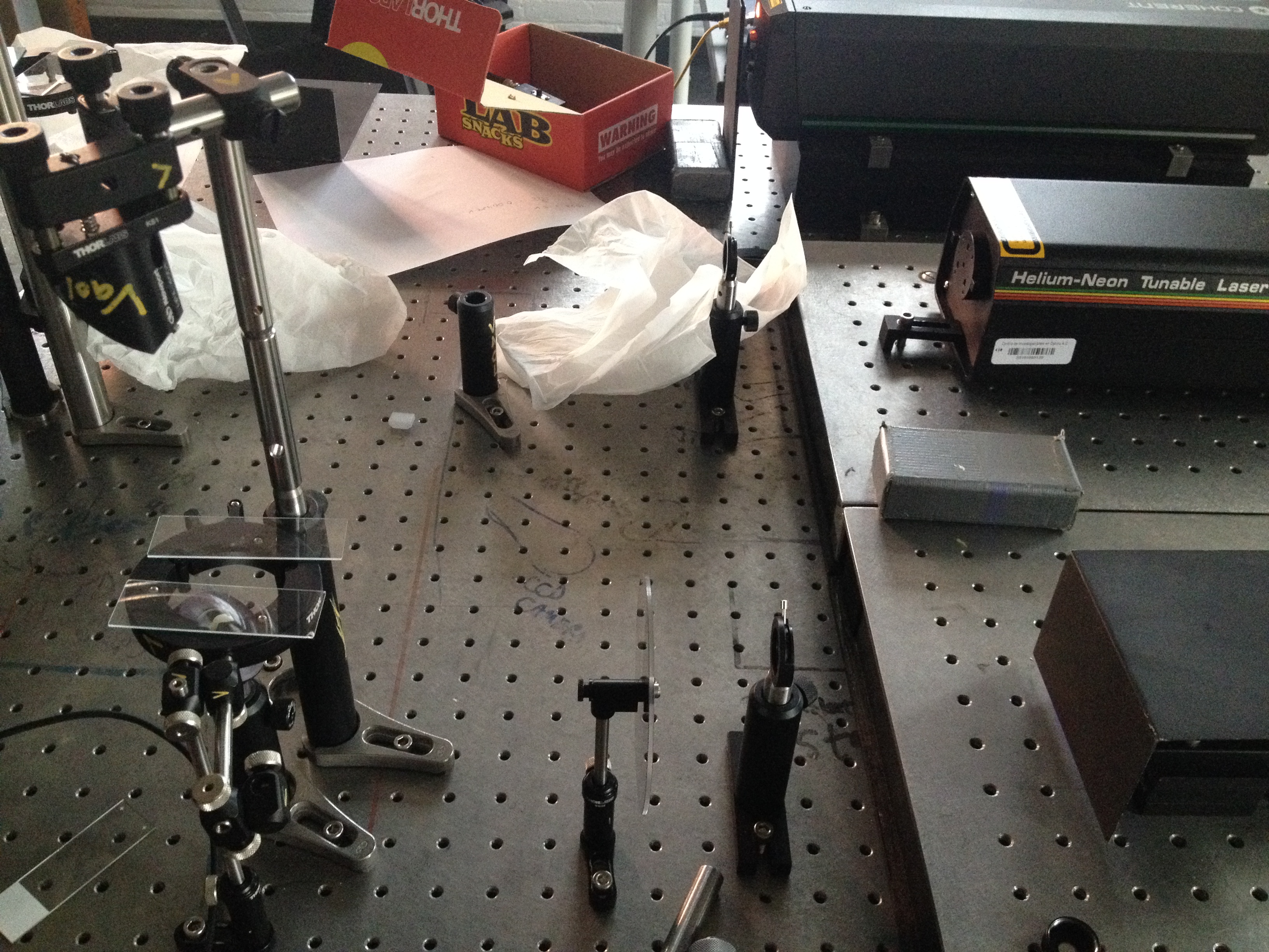
We were able to finish the table set up. It is pictured below. To the left you can see the blue laser. This laser is sent through a pin hole to a mirror that reflects the beam to the right at a beam splitter. The beam splitter sends part of the beam towards the slide holder, and another part to the black shield at the right.
On the right is the Helium Neon laser (red laser). The red laser is aligned to also go through the beam splitter and to the slide holder.
This set up allows us to easily switch between the lasers without having to adjust the set up. A slide will be placed on the slide holder, and as the beam passes through the object on the slide, a diffraction pattern will then be read by a photo diode detector.
This week I also learned how to grow and maintain the C. elegans population we will be using for analysis. This process involves using a microscope to transfer a few mature C. elegans to a new tray with food from a pre-existing non-mutated population. These mature worms will then reproduce and give rise to a new population. The C. elegans are on a four day maturation cycle meaning that it takes four days for then to mature to adult stage. Therefore we have to repeat this process four days prior to when we want to use the worms in the lab in order to ensure they are at the correct cycle for analysis.
If all goes well, next week we may be able to start collecting actual data!
Week 1
Hi everyone! I would first like to introduce myself. I am Trey Cimorelli, a sophomore here at Vassar College. I will be a lab intern this semester in VAOL working mostly on the C. elegans project, and I’m extremely excited.
As this is my first time working in a research lab, the first week was my opportunity to learn the ropes. I have some experience in lab through intro physics and chemistry classes my freshman year, and also some from high school. However the VAOL lab is completely different from anything I have worked with in the past.
We spent last week (unofficial week one) setting up the lab after the move to the new, absolutely beautiful, Sanders Physics building. Many boxes of different instruments and equipment had to be unpacked and needed homes in the lab. After the bulk of the boxes were removed and the lab was semi-organized, the lab table was ready for set up.
Before we began to set up the table, I first had to watch a laser safety video in order to learn how to safely and properly use the lasers we will be dealing with. The lasers we use are for the most part very safe, however for the blue laser we must wear safety goggles. I also had to learn how to handle and clean the optics. This process involves using a piece of lens paper, folding it multiple times with forceps, and then wetting it with a few drops of methanol or acetone and wiping in one direction across the optic piece. Proper cleaning and handing of the optics is necessary to obtain a clear image.
After that we were able to start the table set up. This is a very tedious and time consuming process and we have only just begun to mount the lasers and some of the other pieces (pin hole, mirrors, etc) onto the lab table.
Next we will have to finish mounting the rest of the necessary optics and align the set up. I also have to learn how to handle and grow the worms, and will be continuing to further my knowledge on the equipment and basis of the C. elegans experiment.
Weeks 6 and 7
In the lab for the past couple of weeks we have been analyzing all of the data we have taken. We did this after we have only taken a few tests mainly to ensure that nothing is going wrong with our data setup so that when we take a massive amount of data it is good to analyze.
Most of the time analyzing the data involves clicking on a video in Logger Pro to track the worms’ movement through the cuvette. As you can see in the picture below, I decided the way I wanted to analyze the data was to have the video from both the red and blue halves of the cuvette on the screen at the same time so that I could track the progress of a worm from one half to the other.
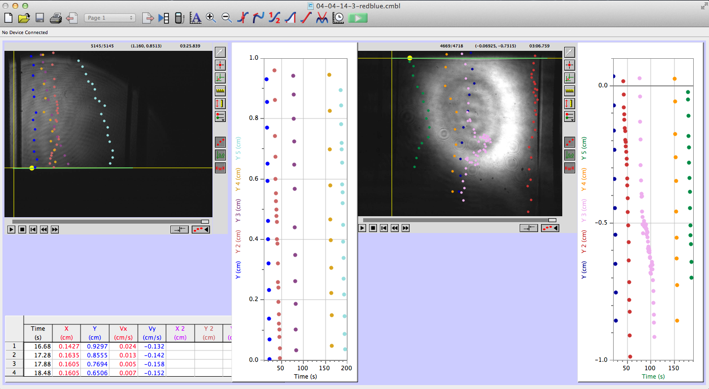
Something odd was happening though where the videos from the blue laser side seemed to take longer to play out and everything seemed to move at a slower pace. Tewa discovered that the frame rate on the blue CCD camera was not set at the same rate as the red; however, a short amount of time in the lab showed that the frame rates can be set on each camera before testing begins, which we will be sure to set at 25 fps from now on
week 6 and 7
“Taking Data”
An expression used by experimenters and scientists regarding the collection and arrangement of data; the steps preceding the analysis of the data.
This week, we took data.
The CCD cameras have proven to be excellent. We drop the worm into the cuvette (through which a green and a blue laser are shining). One CCD camera is trained on the green, and one is trained on the blue.
- Upload the data to the computer, and open the movies in LoggerPro (Insert-> movie-> choose movie).
 “Set Scale” to 1cm by dragging the mouse from one wall of the shadow of the cuvette to the other.
- Set origin at the left end of the “set scale” lin

- Choose options-> movie options-> override frame rate 25f/s and advance by 15f/s
 “add point” and click on the head/tail of the worm. The movie will progress at 15 f/s as you record the entire trajectory
 “add point series” for each new worm to separate data and make it easier to look at.
The whole process is not too difficult to understand, and LoggerPro is relatively easy to navigate. The most difficult part is keeping it organized. For each LoggerPro file, there are two movies (one for each of the colors of laser, one from each CCD camera), and two sets of data (two graphs).
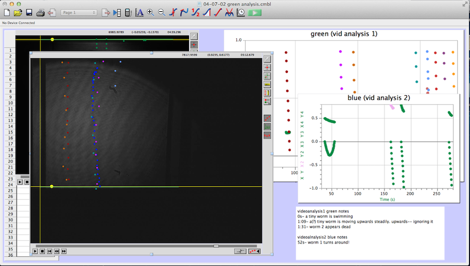
Here is a screenshot of the process. There are two videos open, and two sets of data. I keep note of unusual things that happen during the videos, and label the data sets clearly to minimize confusion. LoggerPro also helps differentiate between the data points by changing the color of each point series (each trajectory is color coded).
What’s next? For now, we have to continue collecting data. In order for a set of data to be at all conclusive or valid, it has to have enough raw data to generate a reasonable average.