Scattering

This page written by Rebecca Eells ’12

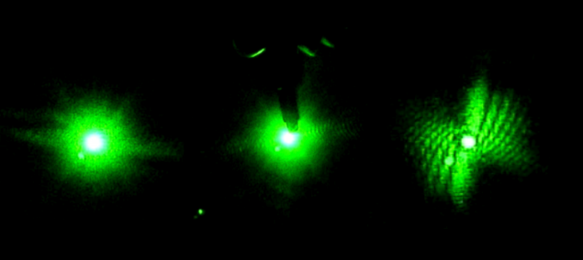
So far this project consists of observing the scattering of laser light by poly latex microspheres.  Eventually this work will build up to being able to predict the size and concentration of small particles.  This can be applied to dynamic systems such that the scattering from C. elegan poop and eggs can be measured and used to determine the size and concentration of the excrements.

5/28/10

Background research was conducted on the different types of scattering.  Rayleigh scattering is observed for tiny particles, less than one-tenth the wavelength of the light.

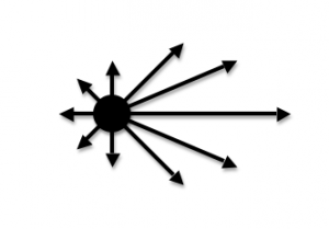
The microspheres are too large in comparison to the wavelength for Rayleigh scattering to be observed. Mie scattering is for larger particles.  A pattern should be produced in which there is more forward scattering than side scattering.  Mie scattering is not wavelength dependent.

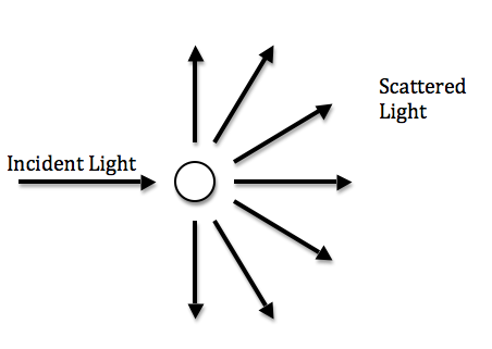
My hypothesis is that Mie scattering will be observed for the microspheres.  The hypothesis can be tested by measuring the forward and 90 degree side scattering of the microspheres.  More forward scattering should be observed than side scattering.  Lasers of different wavelengths can be used to determine wavelength independence.  Statistically similar results should be obtained regardless of the wavelength of laser used.

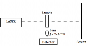
The distance between the laser and the sample is 0.155m for the current set-up.

Three samples were made along with a control cuvette.  The control cuvette consisted of distilled water.  Each sample contained the same volume of distilled water as the control cuvette.  The first sample contained 1 drop 0.11μm microspheres.  The second sample contained two drops and the third sample contained three drops.

Intensity readings were taking measuring the forward scattering and the 90° side scattering.  At this point there appears to be more forward scattering (as expected for Mie scattering) than side scattering.

Another trial will be conducted using the o.11μm microspheres and the red laser to see if the results are the same as with the first trial.  If this is the case, laser of different wavelengths can be used to test for wavelength dependence.

6/1/10

Mie scattering is very difficult to model computationally.  The Rayleigh-Debye theory, which is closely related to the Mie theory, provides an accurate model for light scattering of larger particles and is easier to compute.

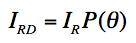
I_{RD=the intensity predicted by the Rayleigh-Debye theory}

I_{R=the intensity predicted by the Rayleigh theory}

P(θ)=a dimensionless form factor

if the spheres are very small then P(θ) goes to one and the equation becomes

6/2/10

The Rayleigh theory of light intensity for scattering by a single particle is:

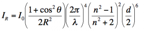
R=the distance to the sample

θ=the scattering angle (either 90 or 180 degrees)

n=refractive index

d=diameter of the particle

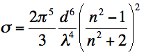
The cross section of one scattering particle is:

6/3/10

An equation is still needed for Rayleigh-Debye scattering for multiple particles.

6/4/10

An equation was found that accurately predicted the scattering intensity of the 0.11μm spheres.  The equation is:

The Rayleigh coefficient is equal to the cross section of the particle (nm²) multiplied by the particle density of the cuvette (particles/nm³).  The Rayleigh coefficient is in units of nm^-1 and accounts for the likelihood of scattering given the particle size and the particle density [2].  The likelihood of scattering also depends on the distance the light must travel through the sample, or the length of the cuvette in nm.  Thus, the Rayleigh coefficient must be multiplied by the length of the cuvette in nm.  This results in a unitless value [1].  But as the light passes through the sample, refraction may take place due to the particles (which is taken into account by the cross section formula) and the background medium (distilled water).  So the refraction of water (unitless) must be included in the formula [1].  The 1+cos²θ term accounts for the phase shift between the incident light and the scattered light based on the angle between the incident beam and the observed scattered light.  Finally the incident intensity is the light that initially entered the cuvette, thus is the maximum intensity of light that could possibly be scattered.

This equation does not take into account the form function, thus can only be used for particles that are small enough to be included in the Rayleigh parameter.

References:

[1] “ECE 532,3. Optical Properties.” Laser Photomedicine and Biomedical Optics at the Oregon Medical Laser Center. 1998.

[2] “Rayleigh Scattering-OPT Telescopes.” Meade Telescopes, Celestron Telescopes and Telescope Accessories-OPT telescopes. 2008.

However when data was taken using 0.5μm microspheres the equation did not yield a theoretical scattering intensity that accurately predicted the observed scattering intensity.  This may be due to an increased particle size such that another term needs to be included.  At first the form factor seemed to make sense, since it only goes to unity for small particles, however the addition of the form factor to the equation still did not yield an accurate prediction.

6/7/10

For the 0.11μm microspheres and the equation above the predicted results are:

Now using the 0.5μm and the keeping the equation the same the predicted results are:

Now taking into account the form factor P(θ) due to larger sphere size, the equation becomes

Using the new equation including the form factor and the 0.5μm microspheres the predicted intensity becomes

While these values are a much closer prediction of the actual intensity, they are not close enough to be an accurate model.  It seems another variable must be included in the equation to account for the spheres becoming larger.  Another option is the equation is wrong entirely.

6/8/10

Another set of data is going to be taken for both the 0.11μm and the 0.5μm.  The volume of each of the “drops” is going to be lowered because the detector appears to become saturated at the 96μl volume.  Also another data set will be taken using the green laser instead of the red laser to see how the wavelength affects the intensity values and the calculation of the predicted scattering intensity.

6/14/10

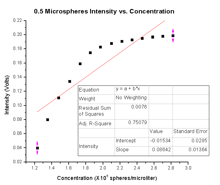
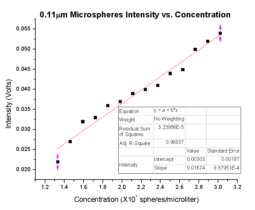
Data was taken for 0.11μm, 0.5μm, and 1.09μm.  Cuvettes with volumes starting at 20μl and going to 46μl were made in 2μl increments.  This data was graphed in Origin to see the relationship between concentration and the intensity of the 90 degree side scattering.

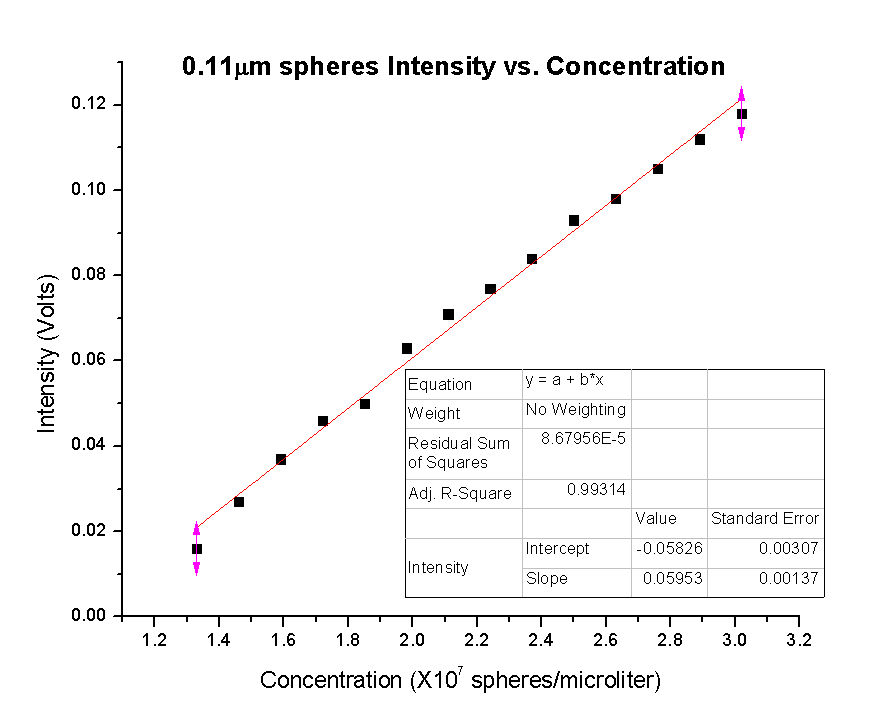
A linear fit was used to fit the data points.  The R-squared value shows that the linear fit was very good, suggesting a linear relationship between intensity and concentration for the 0.11μm microspheres.

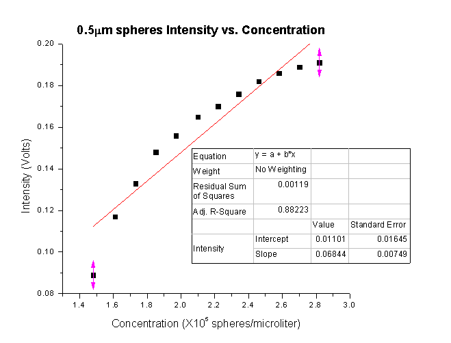
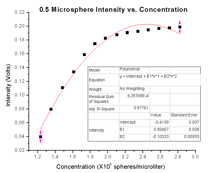
For the 0.5μm spheres a linear fit was first used.  The data points didn’t appear to be linear, but there was a linear relationship for the 0.11μm spheres.  The R-squared value suggested that the fit was indeed not linear.

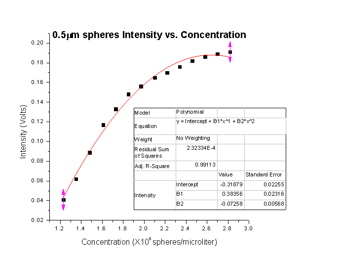
Instead of using a linear fit, the same data points were used with a polynomial fit.  The R-squared value is much closer to one, suggesting the polynomial was a good fit.  The non-linear relationship suggests the increased particle size has led to a more complicated relationship between intensity and concentration.  The larger the particle size, the further the scattering becomes from Rayleigh scattering (linear relationship) and the closer is gets to Mie scattering (more complicated relationship).  Mie scattering takes into consideration interference in addition to the scattering from the particles.

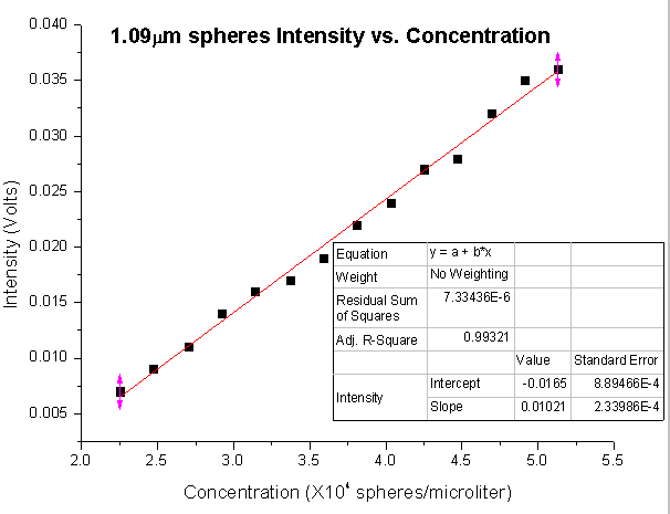
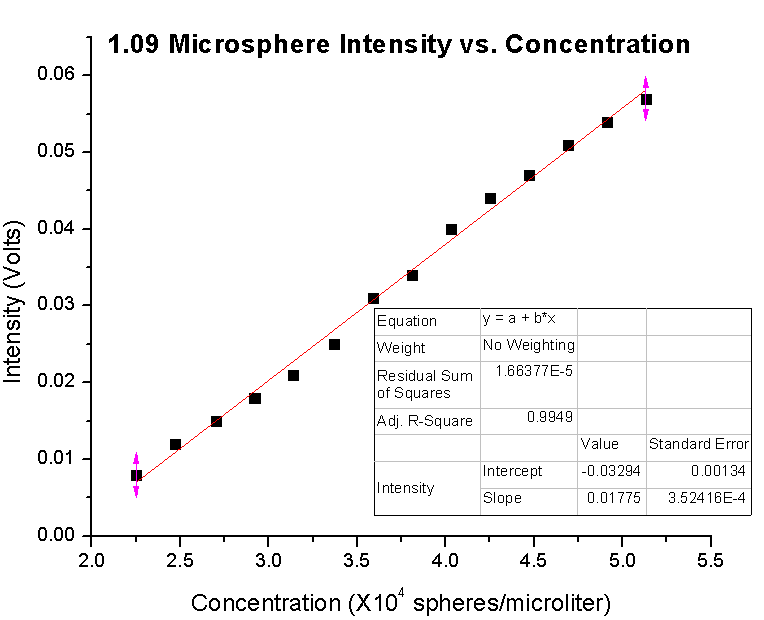
When the 1.09μm sphere data was plotted I expected to see a non-linear relationship between the intensity and the concentration because the particles were even larger and interference should be present.  However, when I did a linear fit to the data in Origin, the R-squared value was very close to one, suggesting the data was indeed linear.

The 1.09μm sphere data may not actually be reliable however.  When preparing my samples, I noticed large white flakes in the solution.  The solution may have precipitated out since the larger sized particles are probably harder to keep suspended.

6/15/10

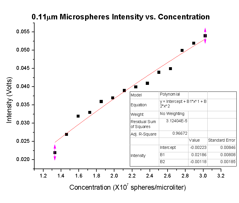
Using the same size spheres and the same concentrations as on 6/14/10, another set of intensity data was collected.  The data was again graphed using Origin.  This time both a linear and a polynomial fit was applied to all the data.

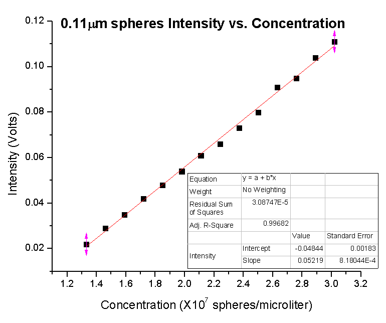
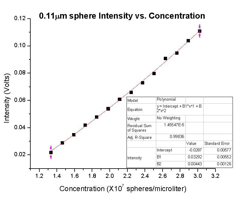
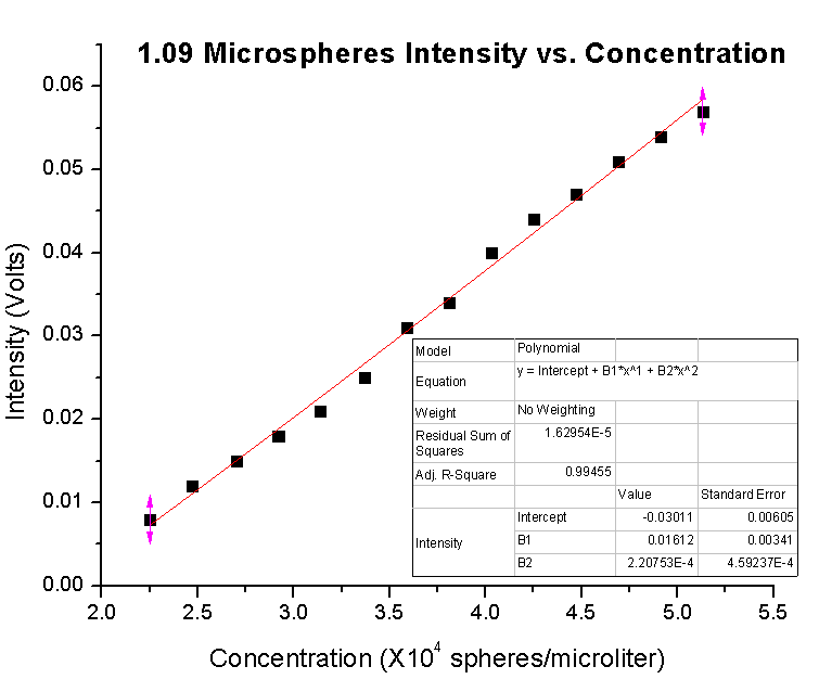
For both the 0.11μm and the 0.5μm spheres the polynomial fit resulted in a better R-squared value (it was closer to one).  However for the 0.11μm spheres, the linear fit did result in an R-squared value close to one, while the 0.5μm spheres the linear fit did not.  This suggests the 0.11μm spheres have an almost linear relationship between intensity and concentration.  It also suggests that the 0.5μm spheres have a non-linear relationship between intensity and concentration.  Only the 1.09μm sphere data resulted in a better linear fit than polynomial fit.  This suggests that the 1.09μm spheres have a linear relationship between intensity and concentration.

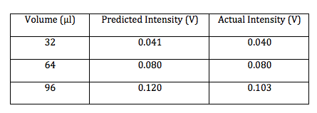
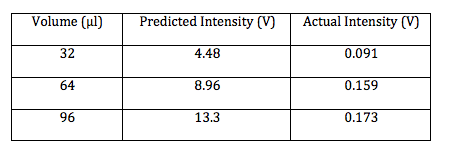
Previously the equation for predicted intensity (above) was used to accurately predict the intensities for the 0.11μm spheres.  Using this equation again and the new data for the 0.11μm spheres, the intensities were predicted.  The table below shows the volume of particles as well as the predicted and actual intensities.

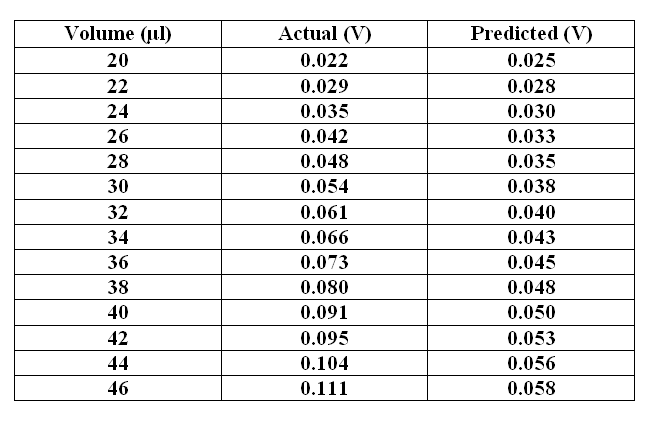
The equation only accurately predicts the first two volumes.  This is strange because before it was used to accurately predict 32μl, 64μl, and 96μl.  Now it does not accurately predict 32μl.  The intensities are much higher for this newer set of data.  Before 32μl resulted in approximately 0.040V of intensity.  Now 26μl results in approximately 0.040V of intensity.  I’m still not sure what would cause this increase in intensity when the volumes, concentrations, and particle size are not changed.

6/17/10

One reason the intensities may have been much higher than expected is that there is a slight amount of error associated with adding the microspheres to the cuvette.  Either more/less microspheres may have been added to the cuvette each time resulting in higher/lower particle density, which affects the intensity of the side scattering.  The data is consistent within itself, based on the R-squared values of both the linear and polynomial fit, meaning the error was either too many particles or too few particles every time.  Since the intensity value was always higher than expected, more particles must have been added to the cuvette each time 2μl were added, resulting in a higher particle density and more side scattering.

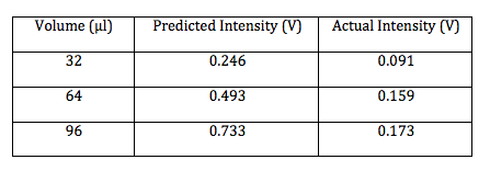
Another data set was taken using the 0.11μm spheres and the same volumes.  However, this time a new cuvette was made for each volume instead of adding 2μl to an original cuvette.  The Origin graphs for both a linear and polynomial fit are shown below.

In this data, the uncertainty associated with the data points wasn’t always high or always low, there was a mix.  This resulted in the data points being harder to fit, thus the R-squared values aren’t as close to one as for the previous data.  However, the intensities are closer to what was “expected” given the equation and previous results.  Below is a table showing the intensities of this data set as well as the predicted intensities based on the equation.

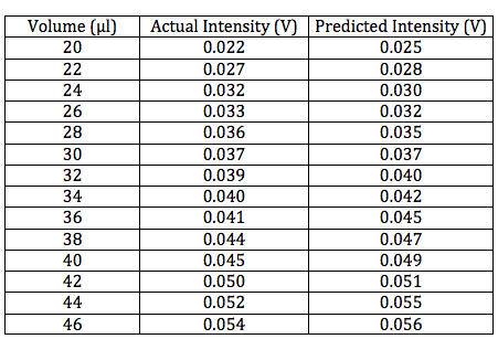
Based on this data, the equation seems to once again accurately predict the intensity for the 0.11μm spheres.  From now on all samples will be made one cuvette at a time, instead of adding volume to an initial cuvette.  Hopefully the high and low uncertainty will somewhat balance out this way.

6/25/10

In Mathematica, a program was written to model the predicted scattering intensity from the 0.11μm spheres as concentration changes.  Below is a polar plot of the predicted intensities as the scattering angle changes from 0 to 360 degrees.  Each curve represents a different concentration of the particles for volumes 20-46μl.

Also using Mathematica, a program was written to animate the graph of predicted scattering intensity.  The animation below shows how the predicted scattering intensity changes as concentration changes for the 0.11μm spheres.

In Mathematica, a program was written to model the predicted scattering intensity from the 0.5μm spheres as concentration changes. Below is a polar plot of the predicted intensities as the scattering angle changes from 0 to 360 degrees.  The formula used to predict the intensities of the larger particles includes the equation for the form factor, which also varies as the scattering angle changes.  Each curve represents a different concentration of the particles for volumes 20-46μl.

The animation below shows how the predicted scattering intensity changes as concentration changes for the 0.5μm spheres.

In Mathematica, a program was written to model the predicted scattering intensity from the 1.09μm spheres as concentration changes. Below is a polar plot of the predicted intensities as the scattering angle changes from 0 to 360 degrees.  The formula used to predict the intensities of the larger particles includes the equation for the form factor, which also varies as the scattering angle changes.  Each curve represents a different concentration of the particles for volumes 20-46μl.

The animation below shows how the predicted scattering intensity changes as concentration changes for the 1.09μm spheres.

7/7/10

An equation was found that accurately predicts the scattering from the 1.09 microspheres.  The equation is:

This equation is the same as the previous Rayleigh equation used for the 0.11 microspheres, except the form factor has been added as well as a constant of one-eighth.  All variables are as previously defined.  Below is  chart showing the volumes, as well as the actual and predicted intensities for the 1.09 microspheres.

7/13/10

As soon as we return from Delaware State University I’m going to take data using the green HeNe laser (wavelength is approximately 543 nm).  Maybe the 0.5 microsphere intensities will be better predicted at this wavelength.  However, the green laser wavelength is even closer to the size of the 0.5 microspheres than the red laser.  Perhaps we will just notice more of the abnormalities in the predictions associated with the 0.5 sized microspheres.  This would still be good, because it’d help add evidence that the abnormalities are being caused by the particle size being approximately the same size as the wavelength.

7/21/10

Instead of using a green laser to take 0.5 sphere data, I used a yellow laser of wavelength equal to 594 nm.  The initial intensity data set was predicted by the Rayleigh-Debye equation I have been using.  I’m going to take another data set to make sure that the data is consistent.

7/22/10

I took another set of data and it appears consistent with the data from the previous day.  Below is a chart of actual intensity and predicted intensity for the 0.5 spheres using the yellow laser.

Using this data a graph was made showing the actual and predicted intensities as well as the error bars and a linear fit.  Both the actual and the predicted intensities have a linear fit, however the fit is better for the actual intensities.  The data set error bars overlap which seems to indicate that the scattering intensity can be predicted using my equation.

I’m also going to redo the graphs of the 0.11 and 1.09 sphere data to include both actual and predicted intensities as well as error bars.  I will also show the charts used to create these graphs.

For both the 0.11 and 1.09 spheres, the uncertainty associated with the actual intensities was a best guess.  Since this data was previously taken there was no way to know the actual uncertainty associated with each data point.  However, the detector very rarely gave readings that fluctuated more than 0.002 Volts in either direction.

Yet again the error bars appear to overlap suggesting that for the 0.11 and 1.09 sized spheres the scattering intensity can also be predicted.