VAOL:Vassar Applied Optics Laboratory – Page 3

Weeks 3 and 4

Due to a whole bunch of work that piled up over the past 2 weeks, I am combining weeks 3 and 4 into one post.

During week 3, Brian showed me a basic intro to analyzing diffraction patterns of c elegans and we spent some time attempting to optimize our optical table. On this blog site there is some data on the diffraction patterns of c elegans and how to analyze them through mathematica. We also watched a video attempting to match the patterns in the video to known patterns on the site to analyze the position and movement of the worms.

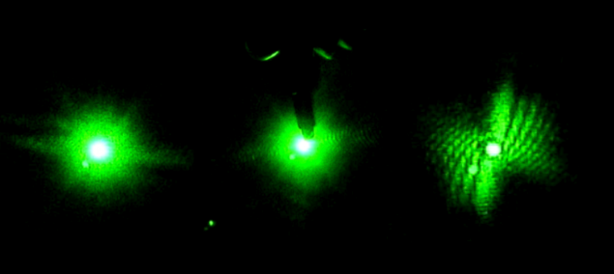
On day 2, we went into the actual lab and attempted to analyze data by dropping worms into the split red/blue laser light. Everything was going smoothly until the worms entered the blue light, where we could only see a small blurry circle on the blue image. We repeated our tests a few times and even on the recording you could not clearly see the worms. This was “solved” just before we left the lab by moving the focusing lens for the blue laser closer in the beam path before the final mirror. This change seemed to help immensely with the focus of the image from the blue laser and we could then, for the most part, tell where the worms were.

When week 4 started we once again didn’t have a lot to do because we couldn’t get into the lab and the worms were not ready to be tested. So instead of any hands on testing, Brian showed me how to analyze data from tests he and Tewa ran earlier in the week. Analyzing seemed kind of simple by just using logger pro to view the videos and clicked where the worms are once every 15 frames. You want to always try and click either the head or the tail of the worm each time and not switch back and forth to get the most accurate data set.

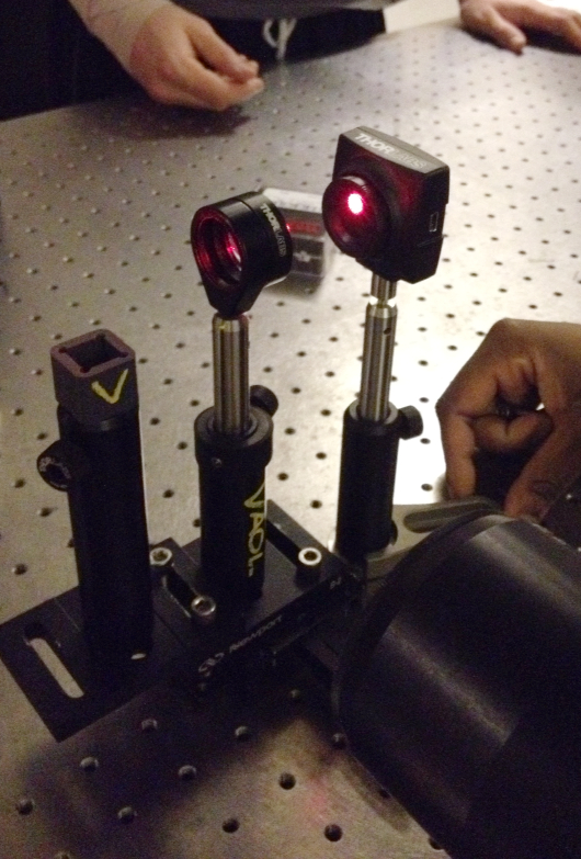
Day 2 started with a meeting with Professor Magnes, where she suggested using a CCD camera to record the data instead of the camera now that just recorded the images. We went into the lab after and immediately began setting up the CCD camera to run some tests. We made sure to not place the receptors for the camera in the most intense point of the beam, but the problem was we were not getting the full image that we needed to test. When we moved the camera farther away to get a better view of the image, the receptors stopped transmitting data. We were in a constant battle between trying to find a working distance for the CCD camera to display data, and the distance needed to see the full image we needed to test.

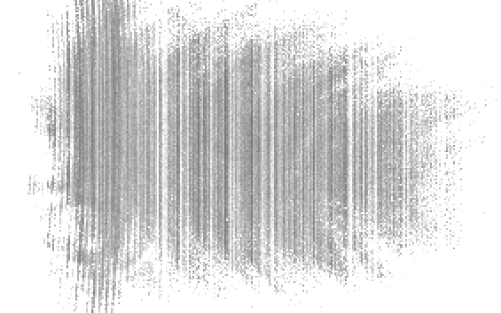
(An image of what the CCD camera was displaying) (Taken by Tewa Kpulun)

Next week we will hopefully get the CCD camera working the way we want it to so that we can record the data accurately. Accurate data is necessary to see if the c elegans have any reaction from the transition from the red into the blue laser light.

week 3

In the lab, things do not go smoothly line to line like in classroom physics problems. Experiments take endurance and patience: you will fail before you succeed.

Current project: Analyzing the C. elegans’ reaction to different light wavelengths (blue and red).

Problem: The videocamera cannot effectively record the nematode’s path through both the red and blue– it is very hard to track its path when analyzing the data.

Proposed Solution: CCD Camera.

CCD camera as it will be placed for data collection (lens cap on)

A “charge-coupled device” camera, although much pricier than a digital camera, converts the light it senses into electrons (just like a solar cell). They then interpret the assembled charge, and transfer the analog data into digital pixels. These cameras produce extremely high-quality images due to the charge moving across the chip with very little distortion.

This particular camera (pictured) is great for the setup because it can 1: be placed directly in the beam to collect images, and 2: plugs into the computer to easily record the images.

What’s next? First we have to confirm that this CCD camera will solve the above problem. Then onto data collection: it is unknown whether the worms react more to green or blue light. It is known that they swim away from UV light. First, collect data for blue and green. Then, on to a UV laser?

Week 2

This week in the lab we did some new things to prepare for actual data taking which we hope to start as soon as possible. I learned how to measure and record data about the optics table, how to set up/move items on the optics table, how to clean optics, and had some hands-on practice picking worms.

The first day this week, Brian brought in a new string to measure the distances on the optics table so that we could record everything in detail in the lab notebook. To measure the distances between the items on the table, I had to hold the base of the string as close to one item without getting oil from my skin onto it, then pull the string tight and do the same with a point in the middle of the string. Once this distance was measure on the string, it was easy to mark the point on the string with a pen then measure the end to the mark on a ruler. I recorded the data so that Brian could put it into his notebook with the detailed sketch of the table.

When measuring the distances for the blue laser, we came across the problem that the beam from the laser was not traveling exactly where we wanted it to. We spent most of the time after that trying to re-align the setup for the blue laser so that the image off of the mirror is as large as possible. By using the holes drilled into the table you can estimate where the beam will be by trying to have the beam run parallel to the holes directly over top of them.

At the end of that day, Brian gave a quick tutorial on different ways to clean optics. My favorite way is the drop and drag method where you put a single drop of cleaning solution on the cloth and drag it slowly across the optic.

The last major thing I did this week was I got to pick worms for a new petri dish. I thought it would be very difficult to have the worms stay on the pick and not fall off during transfer, but they seemed to wrap around the head of the pick and not let go. It was not too bad picking the worms, and I am sure that I will only get better as the semester goes on.

I am looking forward to next week where we will hopefully finish aligning the blue laser and begin taking data with the worms inside the optics lab.

week 2

Learned:

to measure/ record an optical setup
what to do when the setup does not actually function
to clean optics
to pick worms.

This week was the first real week in the lab where I could help instead of being lost.

1) Measuring a setup: Hold a piece of string taught between your fingers. Making sure it is parallel to the table, hold one end directly above the center of the laser lens, and pinch the string directly above the first obstacle (pinhole, lens, etc). Mark the distance with a marker, and measure against a ruler. Record and repeat. Below is an image from my notebook, drawn on 2/13/14, of the Helium-Neon laser setup (from above).

2) What to do when the setup is not aligned: The laser work table is sturdy and covered in a grid of holes, into which instruments can be secured. If the instruments are not in alignment, the laser will not reach through all of the lenses, etc, to reach the screen. To adjust, simply line up the instruments against one of the straight lines of drill holes. Most instruments will either be in a straight line or at right angles to each other.

3) Cleaning optics: Cleaning the mirrors and lenses is essential to get a clear image projected on the screen. To clean: place the mirror on a paper towel (that material does not really matter). Take a piece of lens paper, being careful to touch it as little as possible. Fold it, using the small forcep clamps, until a clean edge can be secured with the forceps. Wet the paper with a drop or two of methanol, and wipe slowly across the mirror, making sure not to touch the mirror with the same section of paper more than once.

4) Picking worms: First, retrieve a 4-day old (mature) dish of C.elegans worms, and a new dish with food (E.coli). Pick a Pick (a glass rod with a tiny wire of on the end). Using the dissecting microscope and a bunsen burner (to sanitize the pick between each contact), move four or five worms from the old plate to the new one. This is difficult at first because depth perception through a microscope takes practice and patience. Try not to kill any worms. Then wrap the dishes, mark them “VAOL” and the date, and place back in the refrigerator for four more days.

In conclusion: Some big strides were taken in the lab for me this week. I am looking forward for the data collection process, which is scheduled to begin on Monday (2/17).

Week 1

As the other new grunt of the VAOL, this first week was spent learning the ropes around the lab. I started out my week watching a laser safety video so I would be allowed to go into the actual lab where the lasers are kept and where all of the testing will take place.

Brian also showed me the worms (C. elegans) that we will be growing and did his best to explain the process of moving the worms onto a new petri dish with a fresh supply of food so that they can lay eggs and make more worms to work with. It takes 4-5 days for the worms to mature into adults, which is when testing occurs and the optimum time to move them onto a new dish.

Another good part of the week was spent assisting our professor with some tasks she needed to get done, including testing multiple pieces of data recording equipment. Spending time to make sure everything is getting done in the physics building is a necessary part of the research assistant position I am in.

Next week Brian and Tewa will teach me how to move worms into new dishes without hurting the worms or the gel that they are placed on. I am looking forward to it!

week 1

As one of the new grunts of VAOL, this first week has progressed appropriately awkwardly, full of disorientation and demonstrations. I think it is appropriate to keep this first post simple, and avoid technicalities.

As I’ve been introduced to the lab, several themes have been repeated to me:

Experiments usually fail several times before any actual progress is made. One step back before two steps can be made forward.
There is a lot of waiting involved. In order for science to be done, there is a lot of shuffling around and communicating to be done first, then purchasing of equipment/setting it up, then figuring out what experimental procedure will answer the proposed question, etc. In this case, working with C. elegans, an additional step is figuring out how to coordinate the work with a living creature, and how to best make due with the supplies at hand.
A good understanding of the equipment is essential. As an example, in the current Shadow Imaging experiment, a Helium-Neon laser is the most useful laser because the beam is safe (easy to work with), it is relatively affordable, has good beam quality (stays focused for an extended time), and it has an adjustable wavelength, and as a result, can efficiently produce any wavelength of visible light (unlike many other types of laser). In general, it is extremely important in experimental setup to do thorough research on what type of equipment would be best for the experiment long before the actual experiment can be conducted.
There are often simple solutions to complex problems. For example, also in the Shadow Imaging experiment, one problem that arises is: how to keep track of the beam’s magnification on the screen? Simple solution: set a clear ruler at the measuring distance between the laser and the screen , an mark on the screen the magnification. In a word, good experiments require some Cleverness.

What’s next? –> I will soon be learning how to grow worms! The almost-microscopic C. elegans has a reproductive life cycle of about 4 days, and to keep the population constant, they must be transferred from dish to dish to give them food and a fertile location to reproduce. Apparently, it takes practice to learn to do it without killing them…

Welcome to the new VAOL Blog!

Hi everyone! I’d like to be the first to welcome you to the new and improved blog for the Vassar Applied Optics Laboratory!

My name is Ramy Abbady, and I am a rising sophomore (Class of 2016) at Vassar College. I’ve been working at VAOL as part of Vassar’s URSI program (see the URSI website or URSI blog for more information) this summer. In addition to my research, I’ve also been updating and doing maintenance on this and other blogs for Professor Magnes.

Above, you’ll find the new navigation system for this blog. We now have an About page, and past year’s research is found under the appropriate heading. Ongoing research is under its own section, as appropriate. The bios of our team members will be posted under the People page very soon!

Browse around the site! And if you have any suggestions regarding the layout, navigation, or anything else regarding the blog, please don’t hesitate to contact me by email, at raabbady@vassar.edu.

Swimming Frequencies of Freely Swimming C. elegans

Most, if not all, studies of thrashing frequencies of swimming frequencies of C. elegans have been conducted using microscopic techniques. Microscopic techniques require microscopic life to remain in a focal plane within microns. Using microscopic techniques, the C. elegans are therefore ‘slipping and sliding’ on a microscope slide in a water droplet. The worms are then not truly freely swimming since they are making contact with the microscope slide. Using laser diffraction, we found that the average thrashing frequency of swimming C. elegans differs significantly from nematodes on a microscope slide by about 0.3 Hz. Our new article on thrashing thrashing frequencies of freely swimming C. elegans can be downloaded from the Open Journal of Biophysics: http://www.scirp.org/journal/PaperInformation.aspx?paperID=21423

More publications are listed here: http://pages.vassar.edu/vaol/pubs/

Overview of the Iterative Algorithm for Phase Retrieval

In the previous post, the reason that only oversampled patterns can be reconstructed was introduced.

The next question is then–how do we construct these patterns and how can we retrieve the phase quantitatively? Here’s a overview of the iterative algorithm that is popular in the “Phase Retrieval world”, especially for nonperiodic objects.

First, let’s list out a few possible constraints, including the one we introduced in the last post, that we usually apply to the retrieval process to make sure that the phase we get back is what we originally have:

1) Creating known-valued pixels. For example, we could create an object with some non-scattering density (zero-valued pixels) inside it, such as the center of the object. In this method, a concept similar to the oversampling ratio comes about, which is a ratio calculated by “total pixel number/unknown-valued pixel number”. This has to be larger than 2 for the reconstruction, just as the oversampling ratio has to be larger than 2.

2) The previous introduced Oversampling method. Basically, with an oversampling ratio larger than 2, we can create a finite support for the object where the pixels outside this support are all zero, creating zero-pixels constraints again.

3) Apart from the external constraints of 1) and 2), we also have an internal constraint which is the positivity constraint. A complex valued object density can be expressed using complex atomic scattering factor, f1+if2. f1 is the effective number of electrons that diffract the photons in phase, which is usually positive. f2 is the attenuation and is also positive for ordinary matter. So the fact that these two values should usually be positive could serve as positivity constraints for the phase retrieval process.

Now that we’ve learned all the constraints, we should look at how the retrieval method is actually carried out through the iterative algorithm:

1) The measured magnitude of the Fourier transform is obtained through the diffraction pattern. We will combine it with a randomly created phase set and generate a new Fourier transform.

2) This Fourier transform is then inversely fast Fourier Transformed to create a new “image density”.

3) Through the oversampling ratio, a finite support is defined in real space for the separation of the density and no density region. For density outside the support, we enforce it to be 0, and for the density inside, we enforce the positivity constraints. These are usually enforced by the following equations, where f ‘ is the object density before applying the constraints and f is object density after conforming to constraints (which is also the S set). The second line is to set pixels outside the support gradually to zero, and the “f1” “f2” increase at every iteration until both positive.

After these are constraints enforced, we can obtain a new image density f that belongs to S.

4) With the new image density after the enforced constraints, we obtain a new Fourier transform of the image and adopt its phase set while restoring its central pixels to zero (the center of a diffraction pattern can not be experimentally measured). We have a new phase set which we can combine with the magnitude of the Fourier Transform again.

Usually after a few hundreds to thousands of iterations like this, convergence would be complete and we will be able to reconstruct the original image through retrieved phases.

Dummies Intro to Oversampling Phasing Method

Before introducing the concept of oversampling, let’s first talk about an effect named “aliasing” that is just as important.

Aliasing

An example of aliasing can be seen in old movies, especially when watching wagon wheels on old Western films. You would occasionally see the wheels as if they going in reverse. This phenomenon occurs as the rate of the wagon wheel’s spinning approaches the rate of the sampler (the camera operating at about 30 frames per second).

The same thing happens in data acquisition between the sampler and the signal we are sampling.

Nyquist Theorem

A theorem that states the relationship between the acquired data and sampling frequency (rate of sampler) is stated as the Nyquist Theorem. It states that 2 samples per “cycle” of input signal is needed to define it the input signal. Thus, a signal with frequency f can be accurately measure as long as you are sampling it at greater than 2f.

The following picture is a Frequency versus amplitude plot showing an aliased signal, fa, which occurs due to “aliasing back” from the original signal of 70MHz where

R (sampling rate) = 100MS/s
fs (signal being sampled = 70MHz
fN (the Nyquist frequency) = 50MHz
fa (aliased frequency) = 30MHz

Oversampling a signal

Applying the concept of Nyquist Theorem, we can see that oversampling is sampling at a rate beyond twice the highest frequency component of interest in the signal and is usually desired. Because real-world signals are not perfectly filtered and often contain frequency components greater than the Nyquist frequency, oversampling can be used to increase the foldover frequency (one half the sampling rate) so that these unwanted components of the signal do not alias into the passband.

Oversampling an object through diffraction

In the case of sampling an object, the Nyquist frequency becomes the inverse of the size of the diffracting specimen, and the sampling rate is the laser frequency. As suggested in the last post, reconstruction of an image through its diffraction pattern is a very important subject in our current research, and “the phase problem” that was introduced will be closely tied to the the Nyquist Theorem, where the diffraction pattern of a finite specimen has to be more finely sampled than the Nyquist frequency.

According to the oversampling phase method, the method above corresponds to surrounding the electron density of the specimen with a no-density region. When the no-density region is bigger than the electron-density region, sufficient information is recorded so that the phase information can in principle be retrieved from the oversampled diffraction pattern.

Reference Cites:

yoksis.bilkent.edu.tr/pdf/10.1364-AO.39.005929.pdf

http://zone.ni.com/devzone/cda/tut/p/id/3000