This page was written by Dr. Jenny Magnes
DATA MODELING (DIFFRACTION PATTERNS)
We began our summer project by experimenting with a Mathematica file created to take the discrete Fourier Transforms of actual raw images from a microscope of the C. elegans. The image data of the worm was translated into a matrix using a Mathematica function. Since we were using actual images of the worms we knew what shapes the worms were taking as they passed through the beam. This was an improvement over the previous Matlab method where the shapes of the modeled worms were just speculation.

- Still Frame of Worm taken from Blue X10 Video Data
However the resolution of the Fourier Transform image in Mathematica was not as good as we expected, or wanted, thus another method needed to be developed.
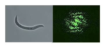
- Example of Worm Image and Resulting Fourier Transform in Mathematica
The matrix created from the image data of the worm needed to be adjusted (made larger) in order to obtain better resolution. The program Origin allows for more control over the matrix. Thus Origin will probably be used to adjust the matrix and then the Fourier Transform will be taken in either Mathematica or Matlab.
———————————————————————————————————————————–
In Mathematica the raw worm image could be turned into a binary matrix. (A matrix of ones and zeros). Based on the threshold value of the image, which is the difference between the background and the worm, the binary matrix could be adjusted to make the values of the worm one and the values of the background zero. (This matches previous worm modeling done in Matlab)
The fast Fourier Transform of the binary worm matrix was taken. The Fourier Transform was squared, the Log method was applied, and the Fourier image produced.
This method gave us the resolution we needed, and we could start using a variety of worm images to match raw video data of the worm diffraction patterns.

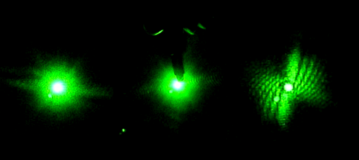
- Raw Video Images

- Mathematica Modeled Diffraction Images

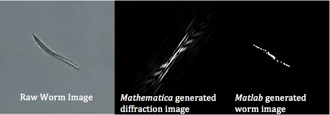
- Raw Worm Images
Based on the size of the beam and the size of the worms we hypothesized that it was possible that many of the diffraction patterns recorded on the video data came from only part of the worm passing through the light, instead of the whole worm passing through the beam. However we had not previously modeled the diffraction patterns of partial worms. Thus using Mathematica, and the technique outlined above, diffraction images from partial worms were generated.
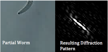
It appears that the resulting diffraction pattern from the partial worm is an even closer match to patterns seen in the raw video diffraction data than diffraction patterns generated by entire worms.
DATA MODELING (WORMS)
The next step for the project was to use Matlab to write a program in which the inverse Fourier Transform of the video data diffraction patterns could be taken. Theoretically the result of the inverse Fourier Transform would be the shape of the worm. (Before we were comparing diffraction patterns taken from the raw video data with modeled diffraction patterns to guess the shape of the worms).
However it was not as simple as just taking the inverse Fourier Transform of the diffraction data matrix. The data matrix created by the diffraction image is the Fourier Transform of the worm squared, or simply the intensity information. Since the Fourier Transform was squared, all phase information was lost. It was necessary to regain the phase information in order to take the inverse Fourier Transform.
In order to regain the phase information, a random phase matrix of the same dimensions as the intensity matrix was generated. The random phase matrix was then combined with the square root of the intensity matrix. The resulting matrix was then squared, which once again eliminated the phase information. (This was necessary to compare the generated diffraction matrix with the original diffraction matrix).

- The squared intensity with random phase matrix
The difference between the squared Fourier Transform matrix and the original intensity matrix was taken to create a new matrix. (I will be referring to this matrix as the difference matrix).
Matrix elements that matched went to zero in the difference matrix. (In our case we only need the elements to be fairly close to zero). For those elements the random phase approximately matched the actual phase. We wanted to keep the elements where the phase matched the same while altering the other elements of the combined intensity and phase matrix. Thus a loop was written in which matrix elements greater than a specified value went through the process of being combined with another random phase matrix while elements in which the phase matched experienced no change. The loop stopped when all matrix elements were less than the specified value.

- The blue color in the images represents matrix elements that are approx. zero.
Note: The loop condition was met when >2*104
The inverse Fourier Transform of the matrix containing both intensity and phase information was taken when the generated diffraction image essentially matched the original diffraction image. (When the image of the difference matrix was almost entirely blue).
First a modeled diffraction pattern from Mathematica was used because the resulting worm shape generated by Matlab could be compared with the actual worm shape used to generate the diffraction pattern. An image of the diffraction pattern was imported into Origin where it was turned into a data matrix. The data matrix was then exported out of Origin and imported into Matlab. The matrix went through the process outlined above and a worm shape was generated from the inverse Fourier Transform. (Worm images were converted into binary images in Mathematica).
Since it appeared, based on Mathematica modeling, that the diffraction patterns in the video data were created by partial worms passing through the beam, the inverse Fourier Transform of a partial worm diffraction image, generated in Mathematica, was also taken. This way when the actual video data was used there was a control for what the inverse Fourier of a partial worm diffraction image should look like.

Finally video data was used to generate worm shapes for observed diffraction patterns where the shape of the worm was unknown. The diffraction images were taken from Cuvette 1. A sequence of eight consecutive diffraction images was used.

As you can see in the above image, only part of the worm was in the beam. The motion of the worm can be tracked by how both the diffraction pattern and worm shape change as time progresses.
The next step is to increase the resolution of the resulting worm images.
AUTOMATED DATA COLLECTION

- Set-up for Automated Data Collection
The oscilloscope used in our set-up connects to the computer for more convenient data collection. The photodiode being used is a high-speed detector that is capable of detecting the rapidly changing intensity of the diffraction pattern.

- Diffraction Pattern Waveform taken from Oscilloscope Data
When a worm passed through the laser beam large, sharp intensity peaks were produced. (An example of the sharp peaks is shown in the image above) The data from these peaks could be exported into an Excel spreadsheet. By analyzing the graph, and searching for the well-defined peaks, sections of the data were extracted and fitted in Origin.

- Origin Graph of Intensity vs. Time with a fitted sine function
The general equation of the sine fit is given below:
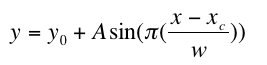
Origin gave a value for each variable. The one we needed to calculate the thrashing frequency was w.
We used the formula:

to calculate the thrashing frequency. We used both previously calculated values of thrashing frequency, as well as the knowledge that for each thrash the worm does, the diffraction pattern has the potential to go through the photodiode twice. (Whether or not the pattern actually goes through twice depends on the shape of the worm).
We collected data for 1mm, 2mm, and 5mm sized cuvettes so that we could control how much space the worms had to move, and so we could compare our frequency findings with the previous frequency calculations from the video data. The data was then compiled and an average thrashing frequency was found for each cuvette size.
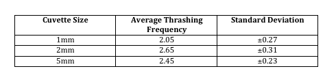
These frequency values are what we expected based on the video analysis. The frequency for the 1mm cuvette does not fall within the std. deviation of either the 2mm or 5mm cuvette. We expected this because the worms can actually touch the sides of the 1mm cuvette, thus they appear to be slipping rather than swimming. For the 2mm and 5 mm cuvette their motion is not constrained by the sides of the cuvette, thus these thrashing frequencies appear to be the frequencies at which the worms swim.
In the future the cuvette sizes may be increased to even wider than 5mm since it appears for our initial data that the thrashing frequency reaches a maximum in the 2mm cuvette and then begins to decline. However with the data we have we cannot assign a trend to what would happen in even larger cuvettes.