Category Archives: Spring 2014

Final Data and Conclusion: Scattering in the Interstellar Medium (ISM)

The goal of my project was to explore a relatively well understood model for light scattered off spherical particles in the interstellar medium (ISM): Mie theory. Over the course of my investigations I switched my inquiry from attempting to derive and plot the asymmetry parameter, g, to plotting the extinction efficiency $Q_{ext}$. Note: I have included portions from my preliminary data post in order to maintain clarity and continuity. Portions from the preliminary post are still relevant and will remain likewise.

Final Reflections

An important question emerges in the study of scattered light in the interstellar medium (ISM). Why use the Mie solutions to Maxwell’s equations as opposed to the Rayleigh or Debye methods for modeling this scattering? As with many other methodological decisions, the answer lies in the physical parameters and observational requirements of the system that I’m trying to model. Optical observational data of extinction due to dust grains as a function of wavelength is denoted by: $A_\lambda$ and this observed data necessitates that the extinction be inversely proportional to wavelength:

$A_\lambda\propto\lambda{^-1}$

i.e. the wavelength must be approximately the size of the grains in question. Only with that dependency will the the model fit the data. Wavelength dependencies for Rayleigh and Debye scattering do not provide the necessary proportion.

Asymmetry parameter, g

As indicated in my preliminary data, modeling the Mie solutions to Maxwell’s equations for scattered light by spherical particles has proven tricky. Ultimately my attempt to plot the asymmetry parameter, g, was unsuccessful, but I was able to plot another grain property instead, the extinction coefficient $Q_{ext}$, versus dimensionless size parameter x (which I will explain in a later subsection of this post). My Mathematica code for the asymmetry work is attached at the bottom of this post as it was in the preliminary data post, but I updated the notebook since I commented on those results and have concluded that work with a derivation of the scattering coefficients $a_n$ and $b_n$.

Below I detail my journey through the asymmetry parameter, g, within of through Mathematica 9 and the processes that comprised those investigations. I find that detailing where I made it up through is important in the process of fixing my work in the future, in addition to being a pedagogically useful process (learning through mistakes!).

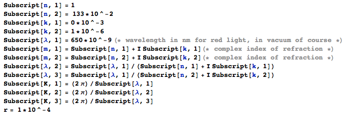
I made some simplifying (and yet physically relevant) assumptions. The spherical grains will be water ice with an index of refraction of n=1.33. The vacuum will have an index of refraction of n=1. Items [k, 1] and [k, 2] are coefficients for the imaginary portion of the indices of refraction. I have assumed a wavelength within the optical spectrum. [K, 1] – [K, 3] are the wave numbers for the different indices and included are the wavelengths necessary to derive those wave numbers. Lastly I have provided an arbitrary, placeholder grain radius.

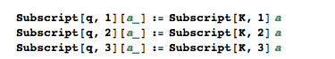
I have also defined grain size parameters, necessary for the calculation of the coefficients $a_n$ and $b_n$, shown below.

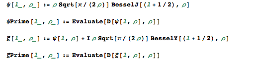
Helpfully, Mathematica has Bessel functions built in. I used them in my exploration into modeling the asymmetry parameter. Dependent on interstellar grains properties, i.e. if it’s dielectric and thus has a real index of refraction or it has a complex index of refraction (impure water ice grain), the Bessel or Ricati-Bessel function will change.

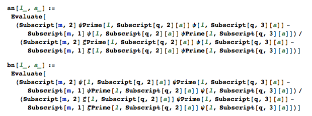
Lastly, here’s my code for the coefficients, $a_n$ and $b_n$. $\alpha$ and $\beta$ have been replaced with q, but those values are still the size parameters.

$Q_{ext}$ v. Size Parameter

In exploring scattering within the interstellar medium (ISM), it is possible to define an extinction efficiency $Q_{ext}$. This efficiency is dependent on index of refraction, m, and can be approximated by

$Q_{ext}\approxeq(8/3)x^4|{\frac{m^2-1}{m^2+2}}|^2$

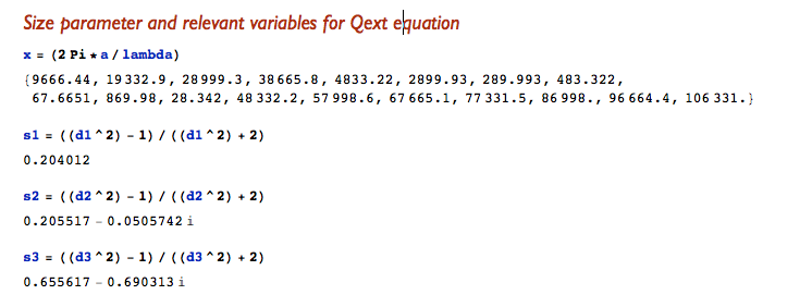
where $x=2\pia/\lambda$ and is the dimensionless size parameter, depending on grain radius, a.

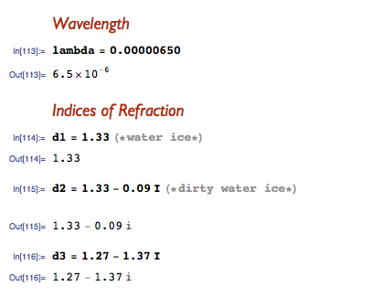
In Mathematica I began by defining a wavelength (red light in microns) and the indices of refraction. Note that indices $m_2$ and $m_3$ (denoted by d2, d3) involve complex components. These components are necessary because of the nature of the grains, which in this case I assumed to be made of different ices.

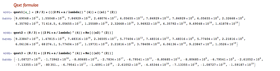
Next I defined the size parameter, $x=2\pia/\lambda$ as well as interior terms for the $Q_{ext}\approxeq(8/3)x^4|{\frac{m^2-1}{m^2+2}}|^2$ equation; specifically, I define ${\frac{m^2-1}{m^2+2}}^2$.

Next I combined the previous bits of Mathematica code to get the actual values for $Q_{ext}$

and then applied a transpose on my data points (where x-values need to be the size parameter, x, and y-values need to be $Q_{ext}$) to be able to ListPlot the three $Q_{ext}$ v. size parameter plots. Transposes shown below!

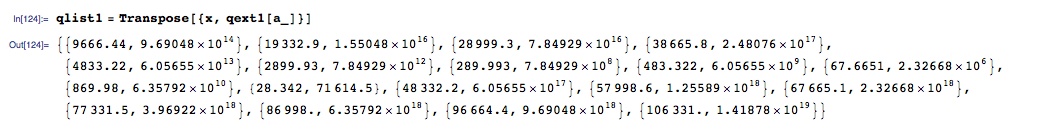
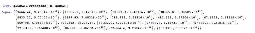
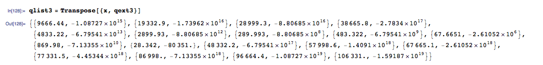
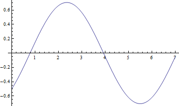
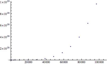
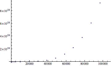
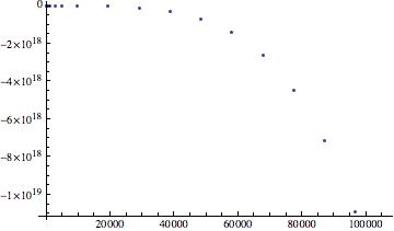
Now I could create my plots! Note that the scales are arbitrary, what I am interested in is the behavior of the plots. This behavior dictates differences in ice grain extinction efficiencies dependent on size and index of refraction. Below are my three plots:

Qext v size parameter x (m = 1.33)

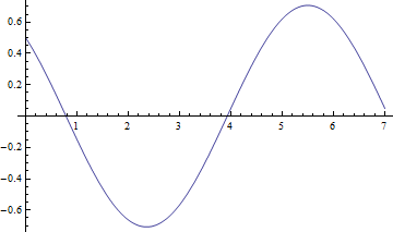
Qext v size parameter x (m = 1.33-0.09i)

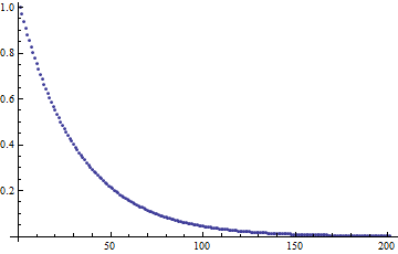
Qext v size parameter x (m = 1.27-1.37i)

Conclusion

While the plots for Qext v size parameter x for m=1.33 and m=1.33-0.09i show a positive exponential trend, the final plot shows quite the opposite behavior. For grains with indices of refraction that have complex components, extinction efficiency versus size parameter plots should indicate a damping in the plot. So I do have some confusion with my plots. The third plot clearly indicates a variation in behavior when compared to the first two, but the second plot (of an extinction efficiency involving a complex index of refraction) should behave similarly to plot 3, not plot 1. This is a good transitioning point into where this work could go in the future – examining whether or not the extinction efficiency versus size parameter plots were indeed done correctly. Mathematica is lenient neither in syntax nor its learning curve! In the future it would also be useful to try and continue my work on the asymmetry parameter, but that might take a greater commitment than just fixing what may be incorrect with the extinction efficiency plots.

I have learned a great deal over the past few weeks about research and computational modeling. I have truly grown in respect to my appreciation for modeling and all the hiccups and hurdles that come with learning how to effectively and efficiently use Mathematica. While my explorations into the asymmetry parameter, g, were unsuccessful at producing a plot, I am very proud at being able to produce plots of extinction efficiency $Q_{ext}$ versus size parameter, x. The results, while not ideal, still reflect trends in the physical behavior of the system – in this case the light scattered by spherical particles in the interstellar medium (ISM).

Resources

Introduction to Electrodynamics, 4th ed. by David J. Griffiths
Physics of the Galaxy and Interstellar Matter by H. Scheffler and H. Elsässer
Interstellar Grains by N.C. Wickramasinghe
Physical Processes in the Interstellar Medium by Lyman Spitzer, Jr.
The scattering of light, and other electromagnetic radiation by Milton Kerker
Mathematica 9 Help Documentation Center (the most valuable resource!)

Mathematica notebooks:

https://drive.google.com/file/d/0B_r-c0PTUHZldHVNREtrWHlzZXc/edit?usp=sharing

https://drive.google.com/file/d/0B_r-c0PTUHZlNVh5emxudUJrRDA/edit?usp=sharing

Final Results and Conclusions: Modeling E and B Fields of a Toroidal Conductor to Explore Tokamak Plasmas

I have developed expressions for B, H, and M for the JET tokamak, and have plotted these fields. I began by deriving the expression for the magnetic field of such a system, approximating it as a toroidal solenoid. I followed Griffith’s example 5.10 to arrive at my expression. As mentioned previously, the expression for the magnetic field of this system is:

$\textbf{B(r)} = \frac{\mu_{0} N I}{2 \pi s} \hat{\phi}$.

As mentioned previously, I use the parameter values from the JET project, and will assume that $N = \alpha q(r)$. My first instinct (and the first value of alpha that I tried) was to set $\alpha$ at the circumference of the torus (17.9 m). As will be discussed below, this did not give reasonable results, and I revised the value of alpha accordingly.

I defined a field (bfield) based on the expression I derived. This was in spherical coordinates since that was easiest to use with the Mathematica command TransformedField. I then transformed this to Cartesian coordinates, and used VectorPlot3D to plot the Cartesian vector field. This produced the circumferential field that I expected. It varies only with distance from the center of the torus ring, and curves around the torus.

The magnetic field, as expected, is purely circumferential and its direction alternates as the current changes. The torus has been superimposed on the field to indicate the region where the field is nonzero.

The torus from a different perspective.

I then repeated the same procedure for the Auxiliary field and magnetization, and both produced the fields I expected (both were the same shape but different magnitudes than the magnetic field and the magnetization was in the opposite direction). Magnetization was in the opposite direction of the magnetic field (as expected) because I used the magnetic susceptibility value of hydrogen (since JET used an H or DT plasma) and hydrogen is diamagnetic (as per Griffiths Table 6.1). A tacit assumption here is that this value does not change significantly when the gas is ionized into a plasma. I do not know what effect this would have on my results, but my results should be viewed with this fact in mind.

The Auxiliary field looks very similar to the magnetic field, and, in fact, differs only in that the vectors have different magnitudes.

Note that all of these fields are identically zero for all regions outside of the the volume of the torus. The values described by the vector field only hold for locations where $(R – r/2) \leq s \leq (R + r/2)$. Unfortunately, I was unable to find a way to force Mathematica to either make the vector field zero in this region or two suppress the vectors so that they did not display. Despite this, the field is correct, just over an incorrect range.

The magnetization in the torus, again, has the same shape as the other fields, but opposite sign.

Now, realistically, the current in my expression for these quantities would not be constant, but would vary with time (as tokamaks operate as pulsed, AC devices). This means that $I = I_{0}\cos(\omega t)$. This assumes that that at time zero, the current amplitude is maximum (which is reasonable since the zero point is arbitrary as long as we look at the system sufficiently long after the tokamak operation has begun).

To account for this time dependence, I let $I = I_{0}$ and multiplied in the cosine term. I did this in the VectorPlot3D argument instead of in the definition of my field because the transform would not work with 4 variables. This should not affect the results. I did this for all three fields. As expected, the fields retain their shapes and the vectors alternate direction with current. An example follows, and the rest can be found in the Mathematica notebook:

Magnetic Field Animation

After developing these models, I wanted to use my expression to find the magnetic field at the center of the torus volume. I would then compare this to the established value for JET’s magnetic field, and the difference would speak to the legitimacy of my model and the assumptions I made, specifically the proportionality constant, $\alpha$. The magnitude of the magnetic field as a function is radius was plotted, to emphasize the fact that it varies only with radius and is not constant throughout the torus (since it spans a range of radii).

The magnetic field strength as a function of radius, to illustrate the fact that the field is zero outside of the torus and that the field only varies with radius. Note also that it is not constant within the torus, as there are several radii encompassed within it. The surface of the torus is included to illustrate the region with nonzero field.

The magnetic field strength as a function of radius, to illustrate the fact that the field does vary with radius, which is not necessarily clear from the vector fields. . The surface of the torus is included to illustrate the region with nonzero field.

For $\alpha = 17.9$, $B = 22.6$T. The established value is $B = 3.6$T. This is a percent error of over 500%. Since this value of alpha was simply a first guess to see how the model worked, this extremely high percent error should not be alarming. We can easily find a better alpha. Knowing what B should be, and the other constants, we can solve for alpha and get that it should take a value of $\alpha = 2.85$. This is very interesting because this means that $\alpha = R$ and that $N = \alpha q = R q = (2.85)(3) = 8.55$. A value of 8.55 for N means that there are only about 9 windings of the current around the solenoid. In Griffiths’ example, he specifies that we assume the windings to be “uniform and tight enough so that each turn can be considered a closed loop.” 8.55 turns around a circumference of 17.9 meters is probably not sufficiently tight. As such, this model has shown that is model is insufficient to describe the behavior of a tokamak (which is not surprising). As it is, this results indicate our model is imprecise. It also indicates that, perhaps, the current should be modeled as a set of smaller currents with tighter windings superimposed on each other. The next logical step in this research would be to examine what exactly the effects of this fallacious assumption are, and how best to address them.

I would also like to note that, while my original plan was to also model the electric field of this system. In my research I have not found any mention of the electric field of a tokamak reactor, only ever the magnetic field. I assume that this is because the magnetic field is the source of confinement, and thus more interesting. Since the electric field seems to be uninteresting to tokamak research, and since I have nothing against which to compare my model, I will not be modelling this field.

With this model (assuming that the windings were closed loops) changing q had a relatively small effect. According to the expression for magnetic field, changing q changer the magnitude of the field vectors (they are directly proportional). In my Mathematica animations of this, though, the change in vector magnitude was never actually noticeable. As such I conclude that, while the safety factor plays a significant role in tokamak design, due to the simplifications made in my model, it has very little effect.

While my results (that N is small and that q has a negligible effect) both indicate that my model is not sufficiently precise to model a tokamak, this does not indicate failure. The main thing that can be learned from this is that a tokamak’s magnetic field is much more complicated than that of a toroidal solenoid, as the current is at a large angle compared to the plane in which the torus lies as it travels around the torus. While my model is imprecise and does not take this into account, it can produce the appropriate values for magnetic field, but with a compromise.

The assumption that went into my model (Griffiths’) that the current loops were essentially closed meant that we assumed the current had only z an s components (and no phi component). The fact that N is so small relative to the circumference means that the current loops will be more slanted and will have a component in all three directions. Obviously, this means that the expression for magnetic field will be different. In the derivation, the fact that the current had no phi component meant that terms cancelled out, leaving us with a purely circumferential field. Clearly, in an actual tokamak, this is not the case. While it is unfortunate that my results showed my model to be insufficient for a robust model of a tokamak, it has been very valuable in that it has confirmed and emphasized the complexity of a tokamak magnetic system. It also puts the current state of fusion research in a very clear context – research has been going on since the middle of the last century, and yet no viable commercial fusion reactor has been developed. This seems to make sense considering the complexity of the systems.

—

Here is a link to the Mathematica Notebook: https://drive.google.com/file/d/0B-C9MvBAfmyIc01BdHRRbGxoRW8/edit?usp=sharing

Final Data: Diffraction Patterns of C. elegans (revised)

Listed below are five sets of data (3-7), two images each. On the left is the photograph of the fluorescing worm. To the right is its corresponding diffraction pattern, produced with Mathematica.

First, a few comments:

Notice that each worm shape contains a different symmetry (or lack of symmetry). However, every diffraction pattern is symmetrical. The two images tend to share some symmetrical qualities, as noted below each image.

These diffraction patterns are due to the fluorescing parts of the worm (GFP, or green fluorescing protein). I believe that because of my image manipulation (converting to grayscale and brightening the image significantly), the diffraction pattern is approximately due to the entire worm and not just the fluorescing parts.

On that note, I’d like to discuss the parameters I used for image manipulation and Fourier Transforming.

The Fourier Parameters I chose were {0, 1} . These are the default parameters when using the FT command on Mathematica. I chose them among the three most common by ruling out the other two: {-1, 1} is used for data analysis (which I was not doing), and {1, -1} is used for signal processing (also irrelevant to my project). My choice of parameters specified the conventions I wanted the program to use when applying the transform.
The command ImageAdjust [image, {a, b}] adjusts the contrast of the image by a and the brightness by b. For most of my images, I adjusted the contrast by the same amount, but changed the brightness differently for each photo depending on my judgement.
I divided the images by hand and reassembled them according to the image dimensions, rectangles of dimension {col/2, row/2} (where col = the number of pixels in each column of the image, and row = the same for each row). I could have use the command RotateRight, but I did not figure that out until after I developed this equally effective algorithm.

IMAGE 3

This image has axial symmetry perpendicular to the axial symmetry of the worm. The worm is mostly linear, and so is the diffraction.

(complete file for image 3: book 3 )

IMAGE 4

See comment for image 3.

(complete file for image 4: book 4 )

IMAGE 5

Although this does not have an “inversion center” (the worm does not complete a loop), it is significantly less straight than the first few examples. Correspondingly, the diffraction pattern has an axial symmetry perpendicular to the “axis” of the worm. However, it splays out to a higher degree, indicating that the area of the pattern corresponds with the curvature of the worm.

(full file for image 5: book 5 )

IMAGE 6

This further backs up my hypothesis from image 5. The curvature of the worm is great and the area of the pattern is also large. However, this worm does have a sort of “inversion center.” The diffraction image has an eye in the center, which is different than all of the preceding images. The curvature of the worm greatly effects the produced image, which is not surprising, but the overall shape of the image changes dramatically. With more circular worms, an “eye” is formed in the center of the diffraction pattern, and the pattern here has both some rotational symmetry and axial symmetry. With straighter worms, the diffraction is much more linear, containing only axial symmetry.

(full file for image 6: book 6 )

IMAGE 7

See comment for image 6.

(full file for image 7: book 7 )

Project Plan

Measuring and Modeling Physical RCL Circuits

Purpose and Goals:

The purpose of this project is to demonstrate the difference between theoretical descriptions/relationships of basic LC circuits and experimental values. This is also an exercise in developing a deeper understanding of the theoretical equations governing these relationships. I will record the voltage drop across various components in each circuit and plot them in comparison to the theoretically predicted values. In addition, I will try to answer questions such as “What are the probable causes for deviation from predicted values?”

The first and most simple circuit I will work with is a basic LC circuit:

The DC power source charges the capacitor until it is discharged (via switch) into the right hand circuit. In theory the current should oscillate back and forth between the capacitor and inductor indefinitely if there was no resistance in the circuit. Actual experimental measurements should reveal some resistance due to the wires and components themselves. Below is the start of my derivations for the voltage across each components:

Kirchoff’s Loop Law states that the total voltage drop across the right hand circuit loop should be zero:

$\Delta V_{L}+\Delta V_{C}=0$ (1)

We know that the voltage drop across an inductor is equal to L(dI/dt) and across a capacitor is Q/C:

$L\dfrac {d^{2}Q\left( t\right) } {dt^{2}}+\dfrac {Q\left( t\right) } {c}=0$ (2)

Which can be rewritten as

$\dfrac {d^{2}Q\left( t\right) } {dt^{2}}+\omega _{0}^{2}Q\left( t\right) =0$ (3)

Leaving us with the general solution to this second order differential equation

$Q\left( t\right) =Q_{0}\cos \left( \omega _{0}t-\delta \right)$ (4)

The derivation of the above equations will be more thorough in future posts.

RLC circuit

This circuit is dampened with a resistor, and thus no longer resembles simple harmonic motion, but rather a damped harmonic oscillator.

Kirchoff’s Loop Law now reads

$\Delta V_{L}+\Delta V_{R}+\Delta V_{C}=0$ (5)

$L\dfrac {dI} {dt}+RI +\dfrac {Q} {C} =0$ (6)

Which leaves us with a new second order differential equation

$L\dfrac {d^{2}Q\left( t\right) } {dt^{2}}+R\dfrac {dQ\left( t\right) } {dt}+\dfrac {Q\left( t\right) } {c}=0$ (7)

$\dfrac {d^{2}Q\left( t\right) } {dt^{2}}+\dfrac {R} {L}\dfrac {dQ\left( t\right) } {dt}+\dfrac {1} {LC}Q\left( t\right) =0$ (8)

$\dfrac {1} {LC}\equiv \omega _{0}^{2}$ (9)

$\dfrac {R} {L}\equiv 2\beta$ (10)

$\dfrac {d^{2}Q\left( t\right) } {dt^{2}}+2\beta \dfrac {dQ\left( t\right) } {dt}+\omega _{0}^{2}Q\left( t\right) =0$ (11)

Eq. (11) is the second order differential equation governing the charge on the capacitor as a function of time and thus describing the voltage drop and current through the other components of the circuit.

Predictions

Theoretically I should expect the voltage across the components in an LC circuit to oscillate indefinitely according to simple harmonic motion. I expect that with a real circuit this would not be the case. A physical LC circuit would actually behave as if a resistor was in series with the two components, causing the amplitude of the oscillations to decrease over time. This is because the circuit parts, such as the wires connecting each component, are not ideal and have resistance.

I predict that a graph of the voltage difference over time for a given component will appear as a decaying sinusoidal wave. In other words it should resemble an dampled oscillation.

Methods

I will use a PicoScope digital oscilloscope to measure the voltage difference across the capacitor in the LC circuit. In this way I will both be able to see the voltage the capacitor is initially charged to as well as record the transition from a steady voltage to an oscillating voltage.

Sources, Resources, and Parts Needed

Equipment Needed:

DC power source, AC frequency generator, Oscilloscope, Computer, Multimeter

Parts Needed:

Breadboard; various values of resistors, capacitors, and inductors; switch; wires/alligator clips

Helpful Texts:

Physics for Scientists and Engineers: A Strategic Approach with Modern Physics (2nd ed.) by Randall D. Knight
Introduction to Electrodynamics (4th ed.) by David Griffiths
Data Reduction and Error Analysis for the Physical Sciences by Philip R. Bevington, D. Keith Robinson
Experimentation : an introduction to measurement theory and experiment design by D.C. Baird
Ordinary Differential Equations by Morris Tenenbaum and Harry Pollard
Class notes – Classical Mechanics (PHYS 210), Zosia Krusberg.

Websites:

http://www.digikey.com/schemeit (for creating circuit schematics)

Timeline

Week 1 – April 20th-26th. Acquire all equipment and parts needed for experiment: Talk to Larry Doe for parts and possibly a power source. Talk to David Rishell about an AC signal generator. Setup experiment in Mudd 216 with Prof. Magnes’ oscilloscope, DC power source, and multimeter.

Week 2 – April 27th-May 3rd. Derive equations to predict voltage drop across components to plot on top of collected data. Those equations being ΔV for LC, dampened LC (RLC), and AC driven RLC in series circuit. Collect data on voltage drops across LC and dampened LC circuit components. Plot data in mathematica.

Week 3 – May 4th-10th. Collect data on voltage drops over AC driven circuit. Predict resonance frequency. Define equations governing resonance frequency and find actual resonance frequency of circuit. Plot findings in mathematica. Consider sources of error or causes of deviation from predicted values on all three circuit configurations.

Week 4 – May 11th-17th. Finish data collection and additional exploration/inquiry. Create time dependent plots in mathematica to demonstrate projected vs experimental values.

Place/Logistics

Experimentation and data collection will occur in Professor Magnes’ lab in Mudd 216. Brian and Tewa generally work MWF and can be contacted for access to the lab.

Preliminary Data: Magnetic Field Modeling

In this post I will describing the specific charge distributions that I will be modeling and showing a brief derivation for the formulas I calculated.

Cylinder:

Problem 5.14 of Griffiths’ Introduction to Electrodynamics 4th edition describes a long cylindrical wire of radius a and steady uniform flowing current I over the outside surface of the cylinder. The magnetic field outside of the wire can be easily found by using Ampere’s Law.

$\oint \mathbf{B}\cdot dl=\mathbf{B}\oint dl=\mathbf{B}2\pi s=\mu_{0}I_{enc}=\mu_{0}I$

(1) $\begin{equation*} \mathbf{B}(s)=\frac{\mu_{0}I}{2\pi s}\widehat\theta& : s > a \end{equation*}$

When looking at points inside of the cylinder, or $s<a$ , $I_{enc}=0$ and so we know that:

(2) $\begin{equation*} \mathbf{B}(s)=0& : s < a \end{equation*}$

Combining our two cases in (1) and (2) we have:

(3) $\begin{equation*} \mathbf{B}(s) = \left\{ \begin{array}{lr} \frac{\mu_{0}I}{2\pi s}\widehat\theta & : s > a\\ 0 & : s < a \end{array} \right. \end{equation*}$

This is plotted below using Mathematica.

Cylinder

As expected, the magnetic field follows the commonly known right-hand-rule where the direction of the current curls around the direction of current.

Plane -> Slab :

Problem 5.15 of Griffiths’ Introduction to Electrodynamics 4th edition, a thick infinite slab extending from z=-a to z=a carries a uniform volume current $\mathbf{J}=J\widehat x$ . The magnetic field inside of the slab can found using Ampere’s Law again.

$\oint \mathbf{B}\cdot dl=\mathbf{B}\oint dl=\mathbf{B}l=\mu_{0}I_{enc}=\mu_{0}IzJ$

(4) $\begin{equation*} \mathbf{B} = -\mu_{0}Jz\widehat y & : -a > z > a \end{equation*}$

When looking at point outside of the slab, our $I_{enc}=\mu_{0}IaJ$ , and so,

(5) $\begin{equation*} \mathbf{B} = \left\{ \begin{array}{lr} -\mu_{0}Ja\widehat y & : z > a\\ \mu_{0}Ja\widehat y & : z > -a \end{array} \right. \end{equation*}$

Sphere -> Ring:

After some research and individual work, I have come to realize that the magnetic field of either rotating conducting sphere or a spherical solenoid is very complicated. I decided to simplify the distribution to two dimensions rather than three for now. A sphere can be viewed as a collection of disks or rings, so I derived the formula for the magnetic field of a ring with radius R and steady current I .

By setting our coordinate system at the center of the ring, we know that the horizontal components of the magnetic field will cancel out through symmetry and the principle of superposition, and we are left with only the vertical component. This leaves us with:

$\mathbf{B(z)} = \frac{\mu_{0}I}{4\pi}\int \frac{dl}{\mathbf{r}^2}cos\theta$

where $\theta$ is defined as the angle between the wire and our position vector $\mathbf{r}$ . It follows then that

(6) $\begin{equation*} \mathbf{B(z)}=\frac{\mu_{0}I}{2}\frac{R^2}{(R^2+z^2)^{3/2}} \end{equation*}$

References:

Griffiths’ Introduction to Electrodynamics 4th edition

Mathematica Notebook:
https://drive.google.com/file/d/0B4ANWxS26h4FRE53d0d5aFRaN0U/edit?usp=sharing

Preliminary Data

The first item to be modeled will be the electric field of a sphere of uniform charge density. This will set the basic framework for any fields based off of a sphere.

To start, imagine a conducting solid sphere of some radius “R” that contains a total charge of Q. There are a couple of ways that the electric field of this configuration could be found. One is Coulomb’s Law, given by:

$E(r)= \frac{1}{4\pi\epsilon_0} \int {\frac{\textbf{$\hat{r}$}}{r^2} dq$

Where $ \epsilon_0 $ is the permittivity of free space and $ r $ is the separation between the source and the test.

The other (and far easier) is to use Gauss’s Law, given by:

$\oint _S {\textbf{E} \cdot d\textbf {a} = \frac{1}{\epsilon_0} q_e$

Where $q_e$ is the enclosed charge of a Gaussian surface, $\textbf{E}$ is the electric field. Note that we are also taking a surface integral. All the math looks interesting, but what is a Gaussian surface? A Gaussian surface is an arbitrary surface at some distance from our actual surface (in this case our actual surface is the previously mentioned sphere), that matches the symmetry of the electric field generated by the object in question. What that means is that the electric field of our real object “flows” through the Gaussian surface in the same way it does the real object. Once this surface has been drawn we can use Gauss’s law to solve for the electric field of the object. In our case, the Gaussian surface is a sphere around out real sphere of some radius that is greater than $R$.

Now, because of symmetry, we can make a few nice simplifications. First, since the magnitude of the electric field is constant (the sphere is uniformly charged) $\textbf{E}$ can be taken outside of the integral, leaving the only thing inside to be $d\textbf {a}$. The integral of that is simply “A” but recall that this was a surface integral, so A is the surface area of our Gaussian surface, a sphere, which is simply $4 \pi r^2$.

Now all we have left is

$\textbf{E}\ (4 \pi r^2) = \frac{1}{\epsilon_0} q_e$

Which is easily re-written as

$\textbf{E} = \frac{q_e}{\epsilon_0 4 \pi r^2} \textbf{$\hat{r}$}$

and there is it. The electric field of a sphere (Griffith’s Example 2.2).

The electric field plotted 3D in mathematica:

Next, we’ll find the electric field of a cylinder of length L and radius R with a uniform volume charge density $\rho$. Again, it will be quite a bit easier to determine this using Gauss’s Law:

$\oint _S {\textbf{E} \cdot d\textbf {a} = \frac{1}{\epsilon_0} q_e$

Just like the sphere we draw a surface that matches the symmetry of our object, and since we want the field outside the cylinder, we again choose a surface that has a radius greater than R, which I’ll call r.

Following the same line of reasoning as the sphere, the left side of the equation can be simplified to just the electric field, E, multiplied by the surface area of the surface. The surface area of a cylinder is given by $2\pi r l$ where $l$ is just the length of of Gaussian cylinder. This lets us write:

$\textbf{E}\ (2 \pi r l) = \frac{1}{\epsilon_0} q_e$

From here we need to find a way to express our charge enclosed. The definition of volume charge density is the total charge over the total volume, meaning that total charge is equal to charge density multiplied by the volume of the object. Again call our total charge Q and we know the volume of a cylinder to be $\pi r^2 l$. Taking our radius as R we can now write our Gauss’s law expression as:

$\textbf{E}\ (2 \pi r l) = \frac{\rho\ \pi R^2 l}{\epsilon_0}$

Solving for $\textbf{E}$ yields:

$\textbf{E} = \frac{\rho R^2 }{2r\epsilon_0} \textbf{$\hat{r}$}$

Which is nicely plotted as:

(excerpt from Griffith’s problem 2.16)

Finally, we have the electric field of a bar. The electric field analogue to a bar magnet is whats known as a bar electret. For this type of model, we will assume that the electret’s shape is similar to the more common picture of a bar – that is that it’s length is much greater than its width.

This electret requires us to use something other than Gauss’s Law. In this configuration the electric field is approximately that of two point charges of opposite charge. The electric field of a point charge is given by:

$\textbf{E} = \frac{q}{\epsilon_0 4 \pi r^2} \textbf{$\hat{r}$}$

The plots shown below are of the two points of opposite charge.

and

The mathematica code for these figures may be viewed here: Preliminary Data

Further modeling may show more complex systems build off of the ones shown here.

Preliminary Data, Magnetic Fields and force in a railgun

From Biot-Savart law of a wire in a closed loop can be broken into 4 parts. Additionally, it should be noted that when considering Ampere’s Law:

The displacement current term is expected to be negligible. That is because in order for the instantaneous rate of change of the electrical field to be significant, the power, loop size and switching rate would have to be extremely, large, small and fast, respectively. Furthermore, for a railgun that size, the current term dwarfs the displacement term by several magnitudes, rendering it irrelevant.

Where z is the shortest distance from a point in space to the wire and theta and phi are the angles between the beginning and end of the wire, respectively. Modeling the circuit as four line currents then allows us to break the B field into four components and solve the above equation, yielding:

railgun

It should be noted that L is the distance from the start of the rail to the slug and is time dependent, x is the distance along the rails, d is the separation between the rails and y is the distance from the bottom rail. Combining these terms using the law of superposition gives the total magnetic field at any point within the loop.

Capture

However, since we are interested in the magnetic field on points within the slug, however, we can set x=L and remove the Bback and Bslug term. The removal of these terms originates from the fact that the nonrail sections are far removed from the slug and generate no significant field within the loop. Additionally, the Bslug term can be removed since due to conservation of momentum, the external magnetic field upon the slug can not be generated by the slug. Additionally, in order to ease calculation, we assume the slug is thin in the x direction, so that we do not have to include width considerations in our calculations. Therefore the Magnetic field upon a point within the the slug (hereafter referred to as B) is:

Next, we will calculate the force upon the slug. Using the Lorentz force law, F=I(dlxB). Since railguns are extremely high energy devices, using enormous currents withing the rails while firing, the best way to power these devices is using capacitors. As a result, the current is variable with time as the capacitor discharges. Additionally, as a result of Faraday’s law, there is an emf generated in the loop as the current and loop size vary, which also affects the current as a function of time.

The force direction is determined by the right hand rule between the direction of the current and the B field within the slug. For a counter clockwise current, the current flows in the positive y direction and the B field for all wire components, including the back and slug, point in the positive z direction (out of the page in the diagram), giving a right hand rule direction of +x.

Additionally, the B field described above is for a specific location along the projectile, and as such the B field must be integrated over the width of the slug. The total magnetic force on the slug therefore becomes:

The magnetic force can also be used in Newton’s Second law to solve for the current in the slug. Of course, this is entirely inaccurate, as there are several means for the current to change, including thermal radiation, rotation and voltage gaps between the slug and the rails. These effects are difficult to calculate and not the subject of this project, suffice to say that the most common method of dealing with these forces is to see what portion of the force is lost.

Since L is time dependent, and extremely fluid, the most common way of reducing this equation is to take the spatial terms and group them into a quantity called the inductance gradient. This quantity is the result of the complex induction effects within the circuit, and is dependent upon the waveform of current, geometry of rails, materials of rails and projectile This quantity, however, cannot be determined theoretically. There are not enough governing equations to solve for L. Instead, what papers concerning railguns use are complicated regression models to determine the optimum dimensions for the rails to maximize this inductance gradient, some of which will be modeled using mathematica in the final data. Therefore, the instantaneous force on the slug can be modeled as:

The Current, being modeled by Elias Kim, can then be inserted into this equation to provide an instantaneous force upon the projectile as a function of t, which can the be solved to (hopefully) provide equations of motion for the slug, and at the very least provide a unsolvable differential equation.

In this reduced form, it becomes clear that the most important factor in this equation is the current, which exponentially increases power as it is made bigger. The 1/2 scalar multiple is the result of the common approximation that half of the current in the loop is required to maintain the expanding magnetic fields, and that only the other half produces force. The navy recently tested a gun that fired a 3.2kg slug over mach 7, this gun used over 33MJ of energy.

As for our physical construction, we had some “technical” difficulties with our design and the small issue of it firing a lethal projectile with highly expensive, dangerous materials. As such we are currently working to scale down our design and will construct it and test this weekend, posting the final specifications and results during the final data.

Mathematica Notebook: https://drive.google.com/a/vassar.edu/?tab=mo#folders/0B0K4JjJfDy1fNnE4MHJON0k4TDg

References:

http://web.mit.edu/mouser/www/railgun/physics.html

Elias Kim

http://ikiu.ac.ir/public_files/profiles/items/1295865343.pdf

http://www.livescience.com/7463-navy-tests-incredible-sci-fi-weapon.html

Preliminary Results: Mie Scattering and the Interstellar Medium (ISM)

Reflections

$A_\lambda\propto\lambda{^-1}$

Asymmetry parameter, g

Modeling the Mie solutions to Maxwell’s equations for scattered light by spherical particles has proven tricky. My attempts so far at getting my Mathematica code to work have hit a bit of a snag, with a plot of the asymmetry parameter, g, versus grain size getting stuck on execution of the code (“running”). I am looking into the possibility that I am unable to execute code due to my laptop’s computational strength – a factor that I entirely did not rule into my planning when I laid out my timeline for the project.

Below I’ve laid out my own navigations through Mathematica 9 and the ongoing process of modeling. I made some simplifying (and yet physically relevant) assumptions. The spherical grains will be water ice with an index of refraction of n=1.33. The vacuum will have an index of refraction of n=1. Items [k, 1] and [k, 2] are coefficients for the imaginary portion of the indices of refraction. I have assumed a wavelength within the optical spectrum. [K, 1] – [K, 3] are the wave numbers for the different indices and included are the wavelengths necessary to derive those wave numbers. Lastly I have provided an arbitrary, placeholder grain radius.

I have also defined grain size parameters, necessary for the calculation of the coefficients $a_n$ and $b_n$, shown below.

Part of the complexity and my uncertainty in my code comes in trying to define a complex conjugate function used in the derivation of the Ricati-Bessel and Bessel functions. Below I’ve included the complex conjugate function that I’ve been utilizing.

Helpfully, Mathematica has Bessel functions built in, what I’ve attempted with them is listed below. Note that I am using density as a means of utilizing the Ricati-Bessel functions (wave functions) on a spherical grain. Depending on an interstellar grains properties, i.e. if it’s dielectric and thus has a real index of refraction or it has a complex index of refraction (impure water ice grain), the Bessel or Ricati-Bessel function will change.

Lastly, here’s my code for the coefficients, $a_n$ and $b_n$. $\alpha$ and $\beta$ have been replaced with q, but those values are still the size parameters.

On a side note, this snag has altered my perspective on the nature of computational modeling. I better appreciate the power and growing accessibility to supercomputing.

Resources

Introduction to Electrodynamics, 4th ed. by David J. Griffiths
Physics of the Galaxy and Interstellar Matter by H. Scheffler and H. Elsässer
Interstellar Grains by N.C. Wickramasinghe
Physical Processes in the Interstellar Medium by Lyman Spitzer, Jr.
The scattering of light, and other electromagnetic radiation by Milton Kerker
Mathematica 9 Help Documentation Center (the most valuable resource!)

Mathematica notebook: https://drive.google.com/file/d/0B_r-c0PTUHZldHVNREtrWHlzZXc/edit?usp=sharing

Preliminary Results – Electric Fields of Spherical Objects

My project is going interestingly. Using the equation of a point charge mentioned in my Project Plan, I achieved the following:

I was also able to successfully plot a sphere of radius 5 centered at the origin, using the SphericalPlot3D function in Mathematica 9. Superimposing the two, I achieved the following:

Clearly, however, this is incorrect, as the field lines should begin at radius of 5 (this is a hollow sphere, with all charge q [equal to the charge of an electron] at the surface), according to Gauss’s Law. I am having trouble getting this to work correctly. I have been experimenting doing it in one octant to get a better idea of how the functions work, but I am still stuck.

My trajectory for the next week is to gain a better understanding of vector functions in general and VectorFunction3D in Mathematica so that I can make better progress. My Mathematica file can be found here.

Preliminary Results: Convolution and the Limitation of Mathematica

Update: See Conclusion

My preliminary results demonstrate the convolution of two arbitrary functions. There are two ways of convoluting functions in Mathematica. The first method is through a tool called ‘Convolve’, and the second method is through the product of two Fourier transforms as discussed in the previous post.

Example 1:

In this example I will demonstrate the convolution of two Gaussian functions of arbitrary widths:

$y_1(t)=exp(-9t^2) \qquad y_2(t)=exp(-t^2)$

The first method is simple. Plug in the two equations into the command ‘Convolve’ along with the necessary parameters. When I did this I got the function:

$f(w)=\sqrt{\frac{\pi}{10}}\cdot exp(\frac{-9w^2}{10})$

The second method requires finding the product of the Fourier transforms of the functions, then taking the Fourier transform of the product. The Fourier transforms of the two functions are as follows:

$f_1(w)=\frac{1}{3\sqrt{2}}\cdot exp(\frac{-m^2}{36}) \qquad f_2(w)=\frac{1}{\sqrt{2}}\cdot exp(\frac{-m^2}{4})$

Taking the Fourier transform of the product of these two functions and $\sqrt{2\pi}$ , yields:

$f(w)=\sqrt{\frac{\pi}{10}}\cdot exp(\frac{-9w^2}{10})$

Both methods yield the same result, which is what should happen every time.

Example 2:

In theory any convolution of two functions adheres to the relationship:

${\widehat_{f_{1}\ast f_{2}}} (x)= \sqrt{2\pi}\;{\Phi_1}(k)\cdot {\Phi_2}(k)$

Using paper and pencil and a lot of free time will demonstrate that this relationship is true. In practice, using a computer program to do the work for you could lead to some issues. Mathematica is limited by the sophistication of its algorithms, and convoluting simple functions can only take you so far. In this example I will demonstrate the limitations of Mathematica. Here I will be using the following functions:

$f_1(x)=exp(-x)unitstep(x) \qquad f_2(x)=sin(x)$

The unitstep function is the Heavyside step function which constrains the exponential function to the first quadrant. Convoluting the two yields the following function:

$\frac{1}{2} (-cos(y)+sin(y))$

The second method gave a slightly different result. Taking the Fourier transform of each function, multiplying them together, and then taking the Fourier transform of that function yielded:

$\frac{1}{2} (-cos(y)-sin(y))$

Both methods worked in the previous example, but here there is a sign change. I tried many different combinations of functions, and most of the time the two convolutions did not match. In fact, most of the time the first method did not give a clear result at all. Sometimes it did not compute the convolution, and sometimes the answer was obviously ridiculous. Fortunately, the latter method always gave an answer. To check to see if the latter method is reliable I redid the calculation using actual data points. I could not do the former method in a similar fashion because no such appropriate tool exists.

I used the ‘Table’ tool to give me a set of values from the two functions above. Here are the plots of the two data sets :

Taking the Fourier transform of each function yields complex values, and so I cannot graph those. The plots of the square of the Fourier transforms are not interesting. After going through with the latter method I came up with this plot:

This result is the same as in the previous attempt through analyzing functions. Considering Mathematica is well suited to handle data, and has a large library of Fourier analysis tools, I am confident that this method will provide the proper results for my future work.

Future

My next attempt will be to demonstrate the convolution of two optical filters. Thorlabs provides raw data of the transmission percentage as a function of wavelength for each filter. I will use the latter method to convolute the two filters, an then discuss how one would try to attempt to deconvolute the convolution.

Mathematica Script

https://vspace.vassar.edu/zerogoszinski/Preliminary.nb

Modeling and Experimental Tools with Prof. Magnes

Ideal for getting ideas and feedback on upper level physics tools.