Category Archives: Spring 2012

Results II – How & Why EDS Works

The induction process of the EDS system is depicted in the diagram below:

Figure 1. The principle of electrodynamic suspension. (a) As the upper current-carrying wire loop approaches the lower stationary conducting loop, the magnetic flux through the lower loop increases with time. The induced EMF in the lower loop, and the lagging induced current, are graphed with respect to time below. (b) As the smaller upper loop passes by the larger lower loop, there is no change in magnetic flux through the lower loop, so no additional EMF is induced. Instead, the built-up current in the loop begins to decline, due to the resistance of the wire. (c) As the upper loop moves away from the lower loop, an opposite EMF is induced, with the same magnitude as before, but negative. As a result, due to the loss in current during (b), there is a net negative current (the shaded region) flowing in the lower loop after the upper loop passes. (Reproduced from Jayawant.)

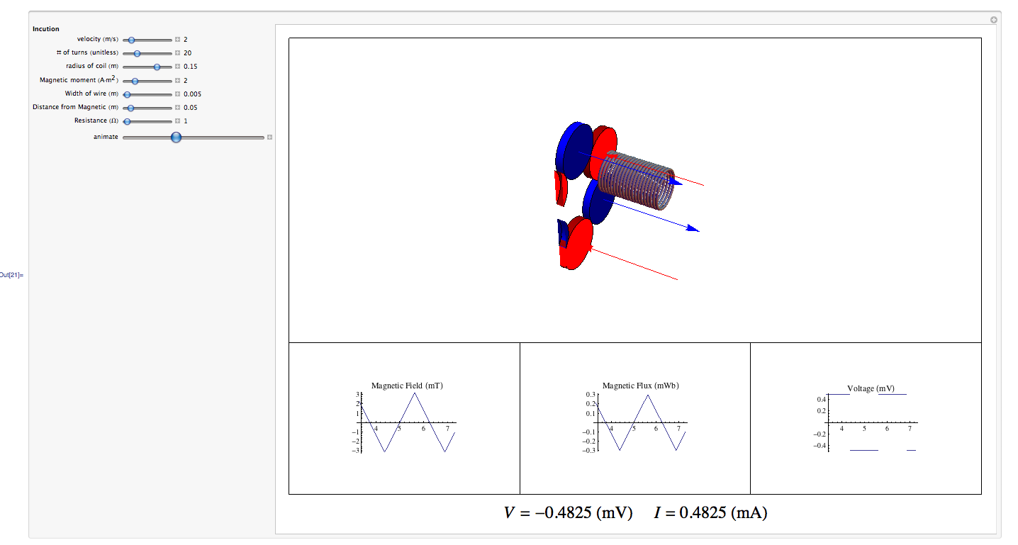
As seen in the figure, there remains an induced current in the lower loop (the conducting track) after the upper loop (on board the train) passes by, flowing in the opposite direction as the current that was initially induced. Thus, this process produces two forces: a lifting force (caused by the opposing magnetic fields generated by the upper and lower loops) and a drag force (caused by the residual current in the lower loop after the upper loop passes, which presents an attractive force on the upper loop in the direction opposite its motion).

From now on, I will focus on finding the relationships between the speed of the train (or, rather, the superconducting coils inside of it), the distance between the train and the tracks, and the magnetic lifting force and drag force that allow the EDS system to function.

Share

Results I – EMS & EDS

So, after having done extensive research into the various types of maglev technologies, I have found that the methods of electromagnetic suspension (EMS) and electrodynamic suspension (EDS) are the most developed and practiced types of magnetic levitation.

As explained before, EMS involves the electromagnets on board the train being attracted to the metallic track from underneath. The current running through the electromagnets is constantly adjusted to maintain a steady distance between the train and the track. One of the easiest ways to model the behavior of these types of maglev systems is by using the equation for magnetic pressure, given as P=\frac{B^{2}}{2\mu_{0}}, from which we can derive the amount of force that the bottom of the train feels towards the track in a given area. However, the main component of this system that changes over time is the current flowing through the electromagnet, which would be extremely difficult to study analytically, and so I will focus on the other main maglev method.

In the EDS system, the electromagnets on board the train induce in a conducting guide way (the track) eddy currents that generate an opposing magnetic field, creating a repulsive force that levitates the train as it moves along the track. This phenomenon is explained by a combination of Faraday’s Law \varepsilon=-N\frac{d\Phi}{dt} and Lenz’s Law. As the train’s superconducting magnets (or current-carrying wires) move along the track, the magnetic field produced by these will move relative to the conducting track, thus generating eddy currents within the track itself. However, these eddy currents flow in a direction such that a magnetic field is produced that opposes the change in magnetic field entering the conducting track. Thus, the magnetic field produced by the train’s electromagnets or coils and the field produced by the track oppose one another, and create the repulsive force that causes the train to levitate.

A simplified model of the interaction between the two opposing magnetic fields is given in the following vector plot. Notice how the two fields interact, opposing one another, resulting in a repulsive force between the two coils that are generating the fields. As the top coil is pulled downwards by gravity, the two fields will interact much more, increasing the repulsion force, and thus levitating the train containing the superconducting coils.

Share

Project Results

Using Griffiths Example 10.3 as a roadmap, I’ve attempted to derive an equation describing the electric potential due to a point charge moving in uniform circular motion. My complete derivation (available here) is too long to post in its entirety, but I’ve outlined it below. It relies heavily on vector algebra, and on a few equations from Griffiths.

First I express a uniform circular trajectory in spherical coordinates:


(1)   \begin{equation*}    \vec{W}(t)=R\hat{r}-\frac{\pi}{2}\hat{\theta}-wt_r\hat{\phi}    \end{equation*}

Then I use Griffiths 10.33 to find an expression for the retarded time. This requires solving the quadratic function in $t_r$, and then making a few clever comparisons (see the full proof) to obtain the correct solution sign. In the end it comes out to be:

(2)   \begin{equation*}       t_r=\frac{ (tc^2-w\phi) - \sqrt{(w\phi+tc^2)^2-\clubsuit(c^2t^2-(r-R)^2+\pi\theta-(\theta')^2}}{\clubsuit}          \end{equation*}

Where I’ve let the $\clubsuit = (c^2-w^2)$ in order to have the equation fit on the page.

I then use Griffiths 10.33 and 10.34 to obtain expressions for the script r vector. In particular, I find a useful expression for the denominator of the Liénard-Wiechert electric potential:

(3)   \begin{equation*}     \scripty{r}c-\vec{\scripty{r}} \cdot \vec{v} = c^2t-\phi wR-(c^2+Rw)t_r     \end{equation*}

Where $t_r$ is defined by equation (2) above. This allows for a substitution directly into the Liénard-Wiechert potential equation (Griffiths 10.39):

(4)   \begin{equation*}        V(\vec{r},t)=\frac{1}{4\pi \varepsilon_0} \frac{qc}{(c^2t-\phi wR-(c^2+Rw^2)t_r})   \end{equation*}

Here I’ve refrained from substituting in for $t_r$ in the interest of space. I’ve created some Mathematica code to plot this derived expression for the electric potential, but I had difficulties exporting it. A quick look at the code reveals why: there are two large regions where the value of the potential is indeterminate. I’m unable to come up with a physical explanation for this, but a mathematical one follows quickly from a look at the denominator of the potential function. Essentially the problem is there exist values of $r$, $\phi$, and $t$ that allows the radicand to become negative, which results in a complex value for the potential. Taking the absolute value does eliminate this problem, but the physical motivation for making such a move is unclear.

As far as the function itself goes, it makes me wonder if there’s not some mistake in my derivation. There are aspects of the physical situation that I feel it models well: the spiral shape, the smoothness near points of maximum potential; for a idea of why the spiral shape is accurate, check out this article, particularly Figure 1 (J.H Hannay, M.R Jeffrey). But the problems are glaring. For one thing, the function isn’t periodic- it drops off to zero for large values of t. Our particle is moving in uniform circular motion, so the resulting potential should reflect that by oscillating as well. The indeterminate regions I mentioned above are also a problem – the electric potential should be defined all regions of the coordinate system. The other issue is that the arms of the spiral cease abruptly after a certain radius- there should be a gradual decrease in potential for larger and larger values of r.

I was able to fix a Mathematica problem that I mentioned in the Preliminary section. One of my animations was exhibiting a suspicious asymmetry, which I discovered was due to an idiosyncrasy of Mathematica’s evaluation. The fixed video is below. It represents the potential due to a point that begins at rest at the origin and moves along the $z$ axis with constant velocity.

Share

Conclusion

Overall I’m happy with my models and analysis for the non-accelerating point charge. The Mathematica animations demonstrate that the equations describe their physical counterparts well, and the proportionality between the electric potential and time for different spacial assumptions was interesting to investigate. Ideally I would have been able to adequately represent the magnetic vector potential field in Mathematica as well.

With more time I’d also try to generate a better model for the circular motion case, whether that means finding a mistake in my derivation or using a different underlying assumption or driving equation. I’d be interested in investigating other particle trajectories as well, perhaps defining more intricate ones but imposing a time-domain restriction.

And of course, there’s always the electric and magnetic fields themselves. To derive the E and B fields for a few simple particle trajectories would be interesting and challenging, and might segway well into some of the material from Griffiths relativity chapter. On page 528 is an alternate derivation for equation 10.68, which is the electric field of a moving point charge. The chapter 12 derivation is described as being both more efficient and more intuitive, and I think it would be worthwhile to take the time to compare the two. Problem 10.15 presents another relativity topic I would have liked to reach: the event horizon. The concept of retarded time is closely linked to any explanation of time dilation or simultaneity,  and I would try to unfold the problem with this in mind.

Share

Jones, Gooch and Tarry, and Transmission

I am going to start out my calculations by writing out the general form of a Jones matrix for TN-LCD as expressed in “Jones-matrix models for twisted-nematic liquid crystal devices” by Makoto Yamauchi:

(1)   \begin{equation*} J = \exp[-i(\phi_0 +\beta_T)]R(-\psi_D)R(-\alpha_T)MR(\psi_D) \end{equation*}

where

(2)   \begin{equation*} \phi_0 = \dfrac{\pi*d}{\lambda}(n_e + n_0) \end{equation*}

and represents the constant absolute phase.

While

(3)   \begin{equation*} \beta_T = \beta\dfrac{d}{2} \end{equation*}

representing the total birefrigence.

The R in equation (1) is the rotation matrix and is represented by

    \begin{equation} \[ R(\xi) = \begin{bmatrix} \cos{\xi} & \sin{\xi} \\-\sin{\xi} & \cos{\xi} \end{bmatrix} \] \end{equation}

And M is the MLC Jones matrix.

We can use this equation in conjunction with the Gooch and Tarry formula in order to help us model the transmission of TN-LCD.

As stated in my Preliminary Data, the Gooch and Tarry formula is written as 

(4)   \begin{equation*} T=\dfrac{1}{1+u^2}\left\{u^2+cos^2\beta{d}\right\} \end{equation*}

Since we will be focusing on TN-LCDs, the twist angle will be 90and the transmission can then be modeled as

(5)   \begin{equation*} T= 1- \dfrac{\Phi^2}{(\beta^2)d^2}\sin^2{\beta*d} \end{equation*}

Here,

(6)   \begin{equation*} \beta*d= \sqrt{\left(\dfrac{\pi}{2}\right)^2 + \left(\dfrac{\pi*d\Delta{n}}{\lambda}\right)^2} \end{equation*}

I then used this variation on the Gooch and Tarry formula in order to graph transmission vs.  d∆n/λ

This graph shows us the first few transmission peaks (Mathematica Code). Transmission operates at 100% when

(7)   \begin{equation*} \beta*d= N\pi \end{equation*}

For N= 1, 2, 3…

Where N stands for the number of wave plates (an LC-cell being thought of as N wave plates).

With respect to our graph, then, the transmission peaks are occurring when

(8)   \begin{equation*} \dfrac{d\Delta{n}}{\lambda}= \dfrac{1}{2}\sqrt{(4N^2)-1} \end{equation*}

This helps us to visualize how the twisted nematic effect operates.

References:

Gooch, C.H. and H.A. Tarry. “The optical properties of twisted nematic liquid crystal structures with twist angles less than or equal to 90 degrees.” Applied Physics Vol. 8(1975): 1575-1584.

Yamauchi, Makoto. “Jones-matrix models for twisted-nematic liquid crystal devices.” Applied Optics Vol. 44.21(2005): 4484-4493.


Share

Conclusion/Overview

Mistakes were made throughout this process. Some were as simple as a dropped variable and others were intensely more complicated. In the end I was still able to produce what I set out to do: An interactive animation that allows you to see how a single coil in a stator of magnetic induction based wind turbine creates current.

Much of the work I did was simply writing the code to get the interactive animation to function properly. Below is a screenshot, but the important code is linked to at the end of this post.

Just to recap some of the derivation I did in earlier posts, I will present a short breakdown here. I started with the basic equation for B, but in order to have the magnetic field change over time based on my magnet array, I had to use a triangle wave. In my previous post I inserted values for the period, but in my Mathematica code, I made it dependent on the velocity so that all the graphs would match up.

Triangle Wave Function:

(1)   \begin{equation*} \frac{4}{d/v}\left [ (t-2d/v)\cdot \left \lfloor \frac{2td}{v}+.5 \right \rfloor \right ]\cdot (-1)^{\left \lfloor \frac{2td}{v}+.5 \right \rfloor} \end{equation*}

Magnetic Field Equation

(2)   \begin{equation*} B=\frac{2\mu }{d^{3}}10^{-4}\frac{4}{d/v}\left [ (t-2d/v)\cdot \left \lfloor \frac{2td}{v}+.5 \right \rfloor \right ]\cdot (-1)^{\left \lfloor \frac{2td}{v}+.5 \right \rfloor} \end{equation*}

Once I had my B(t) I quickly found the flux, but to get to the voltage I had to find the derivative of my triangle wave based B(t) function. I made a square wave approximation to solve for the derivative. In my last post I again plugged in constants in order to show the look of the graph, but in my code I made it dependent on all of the variables.

(3)   \begin{equation*} \frac{4\pi \mu d_{w}rN}{d^{3}}\cdot \frac{4}{d/v}10^{-4}\cdot (-1)^{\left \lfloor \frac{2td}{v}+.5 \right \rfloor} \end{equation*}

Using this square wave approximation I was able to find the voltage in the coil. Once I had a formula for the voltage, the induced current was simple to find.

At this point I noticed a grave mistake with my approach to this problem. By approximating the magnetic field with a triangle wave, I made it so the voltage simply flipped back and forth from negative to positive with no gradation. In hindsight it would have been better to use a version of a sin wave as an approximation. That would present its own issues, as the magnetic field would have a fairly linear change. With more time I would have attempted to find a better approximation for the magnetic field that was easier to use.

It should also be noted that my last post had a few typos in it that could be very confusing. I wrote the equation:

(4)   \begin{equation*} B=\frac{\mu _{0}}{4\Pi }\frac{2\mu^{3}}{d^{3}} \end{equation*}

but it should read:

(5)   \begin{equation*} B=\frac{\mu _{0}}{4\pi }\frac{2\mu}{d^{3}} \end{equation*}

The mu was confused for most of the post, but I was able to correct the issues I had with it for all of the formulas in this post and the code.

Code: https://vspace.vassar.edu/thvandermeer/Trying%20to%20get%20graphs%20in%20it.nb

Share

Limitations of High efficiency

The efficiency of the wave mixing process decreases as $|\bigtriangleup k|L$ increases( although there are some fluctuations). This is becuase when L gets greater than $\frac{1}{\bigtriangleup k}$ the harmonic wave can get out of phase with incident beam and power can flow from the $\omega_{2}$ back into the 2 $\omega_{1}$ waves. The coherence length of the interaction  is $L_{c}=\frac{2}{\bigtriangleup k}$ so the phase mismatch factor can be written as $sinc^{2}(\frac{L}{L_{c}})$

From the phase mismatch plot we see a big decrease in efficiency when $\bigtriangleup k \neq 0$ is not satisfied. This is quite difficult to obtain in labs because the refractive index of materials that are lossless in the range $\omeg_{1}$ to $\omega_{2}$ have normal dispersion when $\frac{dn}{d\lambda}<0$. The refractive index is an increasing function of frequency. For the case of second harmonic $n\omega_{1} = n\omega_{2}$, this is not possible since $n(\omega)$ increases with $\omega$. So what is generally used is birefringence of crystals ie.the dependence of the refractive index on the direction of polarization of the optical radiation. This slows down out of phase waves to get a perfect mismatch.

Share

Conclusions: A look at my model and a look forward to future work

My model is clearly a rough one, and is not entirely accurate to the performance of the average induction generator.  However, I believe that it captures the basic relationships between the variables involved in the operation of a generator, and that the work I have done has the potential to be useful, albeit after some refinement.

Over the course of my work, I have looked into several of models of standard wind turbines, and they have generally focused on the mechanics of the wind and its interaction with the blades, rather than the generator itself.  While the mechanics of this interaction is obviously important to consider when designing a wind turbine, I have been surprised by how little attention is paid to the design of the generator.  It might be said that this is because an induction generator is an induction generator, regardless of where it is, and we already know the most efficient designs.  However, some wind turbine manufacturers are switching to a new gearless design where in place of a gearbox to magnify the rotation rate of the rotor, there is a much larger rotor that can hold more magnets and thus generate more power.  Clearly there are still advances to be made in generator design for wind turbines, and modeling is a good way to explore these potentialities in a cost-effective manner.

If I were to continue my work, the first thing that I would do is construct a more complicated model that accounts for the electromagnetic torque exerted on the stator by the rotor (I believe this to be the largest flaw in my current model).  I would also attempt to look at not just the generator, but the various conversion processes that the generated current must go through before being fed into the grid, as this could inform my design.

Share

Twisted Nematic Effect

A big breakthrough in LCD technology came about in late 1970 when Martin Schadt and Wolfgang Helfrich constructed an LCD based on the twisted nematic effect (Buntz 2). This method employs liquid crystal in the nematic phase that exhibits an angle of 900 in its molecular alignment. The LC-configuration is twisted in a continuous rotation. When the light passes through the LC-cell it is rotated by 900, this allows the light to pass through a second polarizer that is crossed with the first. When a voltage is applied to the LC cell from the electrodes, the liquid crystal molecules align themselves with the field, causing transparency to decrease as the light is blocked when the liquid crystal does not reorient its polarization (Yeh 4). The electrodes applied to the LC-cell are generally made from transparent materials with good electrical conductivity, ITO (indium tin oxide) has been used often in conjunction with LCD screens (Yeh 4).

Super Twisted Nematic Displays came along in the 1980s and differ from TN-LCDs in twist angle and polarizer angle. Instead, STN-LCDs rotate from 1800-2700, while the polarizer angle—instead of 00 as with TN-LCDs—is 450.  The STN-LCDs allowed for more complex pictures. Color Super Twisted Nematic (CSTN) displays use red, green, and blue color filters to create a colored display. Double STN displays stack two STN films with opposite twist in order to achieve a better black/white display. When the color filters are added, the DSTN-LCD has a much wider range of colors than the STN-LCD.

I will be focusing on TN-LCDs as I am particularly interested in the “origin story” of LCD technology and the discovery of twisted nematic effect certainly provided a path for modern LCD improvements.

References:

Buntz, Gerard H. (Patent Attorney, European Patent Attorney, Physicist, Basel). “Twisted Nematic Liquid Crystal Displays (TN-LCDs), an invention from Basel with global effects,” Information No. 118 (October 2005): issued by Internationale Treuhand AG, Basel, Genf, Zurich.

Yeh, Pochi and Claire Gu. Optics of Liquid Crystal Displays. Canada: John Wiley & Sons, Inc., 1999.

Share

Some Applications

I think it is important to talk a bit about the applications of an electro optic modulator. I think some of the modulation applications are fairly obvious. For example, phase modulation is useful when it comes to controlling what time and at what point in its oscillation a light wave will arrive somewhere. Also similar to phase modulation amplitude modulation allows for the control of the intensity.

The main perk of using an EoM as opposed to other less expensive optical elements is the ability to make the voltage time dependent or give it a frequency. The ability to turn the EoM on and off at rapid rates makes for some interesting applications.

One application I am most familiar with is the use of the polarization modulation to pulse a laser beam as shown below

Because of the rapid rate of turning on and off the EoM you get a laser coming out of it that is made up of alternating segments of horizontal and vertical polarization. After you send it through a polarizing beam splitter cube you get two pulsing laser beams.

The length of the pulses is directly proportional to the rate at which you turn the EoM on and off or the frequency which is the amount of times you turn it on in one second. To determine the pulse distance we can use this equation

(1)   \begin{equation*}c=Df\end{equation*}

Where c is the speed of light and f is the frequency at of the EoM

This is very useful to obtain time resolution and filter out noise. Let’s say you have an event that happens in a material and you wish to study it with a laser. If you pulse the laser beam at a known frequency then you are able to only look at events that are happening during the time you know the laser is affecting the material. Like wise you are able to see when it is not affecting the material at the same frequency. This allows you to see events that happen for only a short moment of time within a material.

If I had more time in this project I would do an experimental side, where I use a real EoM to learn more about them. One of the things i would do is determine the size of the crystal inside the EoM by using the phase shift and the known index of refraction. I would also like to assemble the various beam map set ups i came up with In this project and see how effective they are in modulating the laser.


Share