Category Archives: Mathematica

Here is what Mathematica can do…

Preliminary Results: Convolution and the Limitation of Mathematica

Update: See Conclusion

My preliminary results demonstrate the convolution of two arbitrary functions. There are two ways of convoluting functions in Mathematica. The first method is through a tool called ‘Convolve’, and the second method is through the product of two Fourier transforms as discussed in the previous post.

Example 1:

In this example I will demonstrate the convolution of two Gaussian functions of arbitrary widths:

$y_1(t)=exp(-9t^2) \qquad y_2(t)=exp(-t^2)$

The first method is simple. Plug in the two equations into the command ‘Convolve’ along with the necessary parameters. When I did this I got the function:

$f(w)=\sqrt{\frac{\pi}{10}}\cdot exp(\frac{-9w^2}{10})$

The second method requires finding the product of the Fourier transforms of the functions, then taking the Fourier transform of the product. The Fourier transforms of the two functions are as follows:

$f_1(w)=\frac{1}{3\sqrt{2}}\cdot exp(\frac{-m^2}{36}) \qquad f_2(w)=\frac{1}{\sqrt{2}}\cdot exp(\frac{-m^2}{4})$

Taking the Fourier transform of the product of these two functions and $\sqrt{2\pi}$ , yields:

$f(w)=\sqrt{\frac{\pi}{10}}\cdot exp(\frac{-9w^2}{10})$

Both methods yield the same result, which is what should happen every time.

Example 2:

In theory any convolution of two functions adheres to the relationship:

${\widehat_{f_{1}\ast f_{2}}} (x)= \sqrt{2\pi}\;{\Phi_1}(k)\cdot {\Phi_2}(k)$

Using paper and pencil and a lot of free time will demonstrate that this relationship is true. In practice, using a computer program to do the work for you could lead to some issues. Mathematica is limited by the sophistication of its algorithms, and convoluting simple functions can only take you so far. In this example I will demonstrate the limitations of Mathematica. Here I will be using the following functions:

$f_1(x)=exp(-x)unitstep(x) \qquad f_2(x)=sin(x)$

The unitstep function is the Heavyside step function which constrains the exponential function to the first quadrant. Convoluting the two yields the following function:

$\frac{1}{2} (-cos(y)+sin(y))$

The second method gave a slightly different result. Taking the Fourier transform of each function, multiplying them together, and then taking the Fourier transform of that function yielded:

$\frac{1}{2} (-cos(y)-sin(y))$

Both methods worked in the previous example, but here there is a sign change. I tried many different combinations of functions, and most of the time the two convolutions did not match. In fact, most of the time the first method did not give a clear result at all. Sometimes it did not compute the convolution, and sometimes the answer was obviously ridiculous. Fortunately, the latter method always gave an answer. To check to see if the latter method is reliable I redid the calculation using actual data points. I could not do the former method in a similar fashion because no such appropriate tool exists.

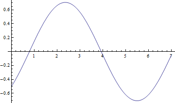
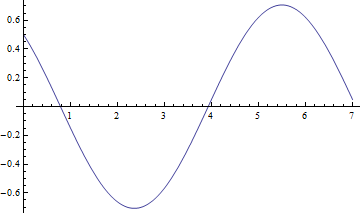
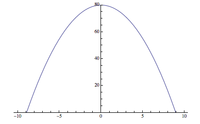
I used the ‘Table’ tool to give me a set of values from the two functions above. Here are the plots of the two data sets :

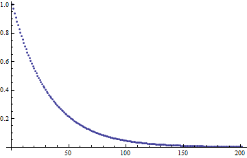
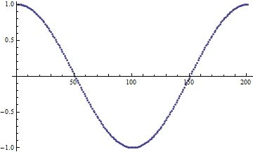
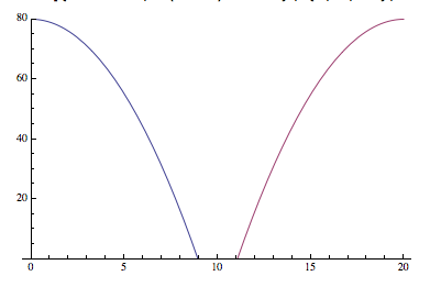
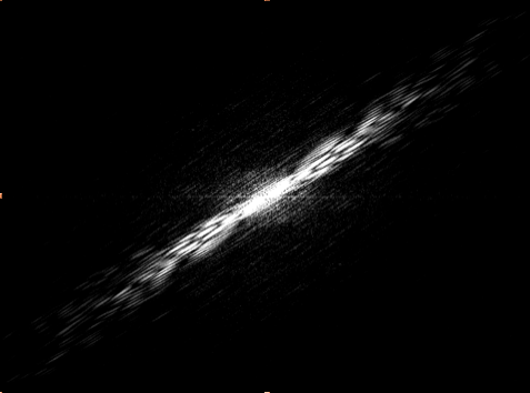
Taking the Fourier transform of each function yields complex values, and so I cannot graph those. The plots of the square of the Fourier transforms are not interesting. After going through with the latter method I came up with this plot:

This result is the same as in the previous attempt through analyzing functions. Considering Mathematica is well suited to handle data, and has a large library of Fourier analysis tools, I am confident that this method will provide the proper results for my future work.

Future

My next attempt will be to demonstrate the convolution of two optical filters. Thorlabs provides raw data of the transmission percentage as a function of wavelength for each filter. I will use the latter method to convolute the two filters, an then discuss how one would try to attempt to deconvolute the convolution.

Mathematica Script

https://vspace.vassar.edu/zerogoszinski/Preliminary.nb

Preliminary Results- RLC Circuits

Overview

In the following blog post, I discuss my progress with my project so far. I start out with a simple RLC circuit, go on to discuss the components, and derive a solution (using Mathematica) for a circuit with parameters that I have come up with. I then plot current as a function of time and discuss long-term structure in the output of the circuit, its relevance to my project, and my forward plan.

Progress

In my plan I discussed a simple RLC circuit that consists of a capacitor, voltage source, resistor, and an inductor. To easily visualize this, I have constructed a basic circuit diagram (Figure 1).

(Figure 1)

The differential equation that governs this RLC circuit is given by

$LI''(t)+RI'(t)+\frac{1}{C}I(t)= E_{0} \omega cos(\omega t)$ [1]

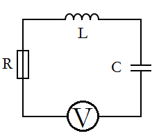
where L is the inductance, R is the resistance, C is the capacitance, I is the current, $\omega$ is the resonant angular frequency, $E_{0}$ is an initial value dependent on the voltage source, and t is the time. The inductance (L), resistance (R), and capacitance (C)are all determined by their respective circuit components, which are easily changed out for different ones. $\omega$ depends on the inductance and capacitance, and its value is given by

$\omega =\frac{1}{\sqrt{LC}}$ [2]

What we have left in terms of variables are current (I) and time (t). For our purposes, time is the independent variable, which leaves the current in the circuit at any time to be the dependent variable. Now that we have established this, we can solve our differential equation [1] for current as a function of time ( $I(t)$ ).

In order to solve [1], I will use the equation solving powers of Mathematica. In particular, the DSolve function is used. When plugged into Mathematica, the input line looks like:

$\text{DSolve}\left[\frac{\text{Current}(t)}{\text{Capacitance}}+\text{Inductance} \text{Current}''(t)+\text{Resistance} \text{Current}'(t)=E_{0} \omega \cos (\omega t),\text{Current}(t),t\right]$ [3]

We must set values for resistance, inductance, capacitance, and $E_{0}$ . For this run through of the solution I chose the following arbitrary values:

Inductance= 1 Henry
Resistance= 10 ohms
Capacitance= .1 farads
$E_{0}$ = 1 Volt

When the command is run with the above values set, Mathematica generates the general solution, which is:

$I(t)=c_1 e^{-8.87298 t}+c_2 e^{-1.12702 t}+0.040824(-Cos(3.162t)+e^{6.661*10^-16t}Cos(3.162t)-0.3564Sin(3.162t)+2.806e^{6.661*10^-16t}Sin(3.162t))$ [4]

First, lets make sure that this solution is reasonable. The known form of the solution to the equation for such a circuit is given by:

$I(t)=c_1 e^{r_{1}t}+c_2 e^{r_{2}t}+Asin(\omega t-\varphi )$ [5]

The form of our equation [4] seems to match up pretty nicely with this known solution [5]. Now, lets examine [4] in more detail.

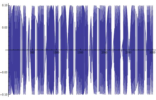
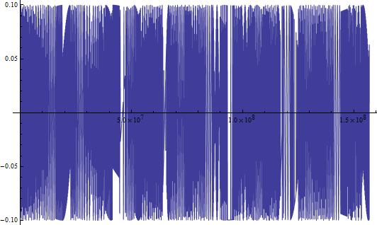
Our solution [4] looks a little daunting, but we can break it down into its components. The first two terms have constants that depend on the initial current running through the system, i.e. when $I(t)=I(0)$ . However, we can approximate the equation by only looking at the last term, which is a superposition of sin and cosine functions along with a couple exponential terms thrown in. The reason that we can apply this approximation is that the first two terms “damp out” quickly, and thus have exponentially less of an effect as time progresses. The reader may still be curious to see how much of an effect these terms have on the current flowing through the system: to that I say don’t worry! After my initial approximation, I will solve for these constants and compare the two cases.

For now, we will deal with the approximate solution, which is:

$I(t)=0.040824(-Cos(3.162t)+e^{6.661*10^-16t}Cos(3.162t)-0.3564Sin(3.162t)+2.806e^{6.661*10^-16t}Sin(3.162t))$ [6]

Now that we have this equation, we can use Mathematica to give us an idea of what the changing current looks like over a longer period of time. Figure 2 shows the current in the circuit as a function of time ( $I(t)$ ) plotted over a 30-second interval.

(Figure 2)

This looks like something we would expect! A sinusoidal wave that describes the changing current over time, just like our equations dictate. But, this is a short time-scale. What happens when we look at the changing current over a longer period of time? In Figure 3, I show the changing current over a longer time period (3000 seconds/50 minutes). In Figure 4, I repeat the process, but with the timescale being 5 years.

(Figure 3)

(Figure 4)

In both Figures 3 and 4, we see some very interesting long-term variations in the current. Why does this occur? Well to be honest, I am not completely certain. I do have a few ideas though:

My first inclination is that the long-term variations are in part due to the approximation I made by removing the first two terms of Equation [4].
My second idea is that these long-term structures are present due to a possible approximation Mathematica may have made when solving the differential equation.
My third and last thought is that these variations are not an artifact of finding the solution, but truly do exist in this theoretical circuit I have chosen.

Why?

A question that the reader may have after looking at all of this is “Why is the long-term structure important?” The answer lies in the fact that RLC circuits are embedded in many electronic devices, including radios and televisions. For this reason, it is important to know the current they put out. We don’t really want something that has an unpredictable output in devices that are high-cost.

Forward Plan

To further investigate the reason for the long-term structure, I will first solve for the constants in Equation [4] and plot the graphs of current again. Hopefully this will provide some insight into the workings of the circuit. I may also alter the initial parameters (inductance, resistance, etc.) to see if this provides any insight. If not, then I will investigate Mathematica’s differential equation solving techniques and attempt to alter my solution in a way that provides a more accurate solution.

Resources

1. Circuit Diagram Maker- http://www.circuit-diagram.org/

2. The RLC Circuit- University of British Columbia- http://www.math.ubc.ca/~feldman/m121/RLC.pdf

3. Mathematica Cookbook by Sal Mangano

Mathematica Notebook

https://drive.google.com/file/d/0B3mtB6CQNnpjejEzN25zbFlqajQ/edit?usp=sharing

Preliminary Data

Using Gauss’s Law for the Electric Field, I found the electric field for a conducting cylinder with a charge density

. (Eq.1)

The end result is the equation

$\overrightarrow{E}=\frac{ks^{2}}{3\epsilon _{0}} \widehat{s}$ . (Eq.2)

With this, I was able to model the following.

(Figure 1)

Here is a photo of what is occurring on the inside of the cylinder. As you can see in Figure 2, the Gaussian surface would be placed in the center of the cylinder where the vector fields start and are directed radially outward. As implied by Equation 2, the electric field is directly proportional to the radius of the cylinder.

(Figure 2)

I am currently working on modeling the magnetic field.

Preliminary Results: C. elegans Diffraction Pattern Modeling

Staying true (so far) to my tentative project timeline, I acquired images of the C. elegans in various shapes, I have done quite a bit of research on Fourier Transforms and Fraunhofer Diffraction, and so far I have successfully transformed one image into the corresponding diffraction pattern.

IMAGE 1

I took this image and used mathematica to sharpen it –> setting it to grayscale and brighten it –> collect dimensional information –> apply a Fourier Transform, yielding (after some similar image manipulation):

This is a great diffraction pattern, but I had issues with the poor resolution and general image quality. To remedy this, I proceeded with images taken with a higher-resolution camera.

(full file for image 1: book 1 )

IMAGE 2

This beautiful image needed some manipulation, similar to image 1: I converted it to grayscale –> brightened it significantly (to make it a more definite shape, and to get rid of the “holes” in the luminescing nematode) –> collected image dimensions and data –> applied the FT. Unfortunately, I ran into a problem.

The produced image:

Obviously this is quite different than the first diffraction image.

I had a few hypotheses:

1. The image was saved as a .jpg, but the same image was produced when I tried again with a .png version of the image.

2. The computer is phase- shifting the image so that instead of the origin lying in the center of the product, it is splitting the right side from the left side and lining them up in the wrong order. How can I rearrange and correct the phase shift in the output?

An analogy to the second hypothesis:

—>

It is as if, instead of centering the origin in the center of the produced diffraction pattern, the computer is putting the “origin” in a different place, and splitting the image, similar to the parabola I produced above.

My solution is a little underhanded. I divided the image into four equal rectangles, and manually rearranged them to produce what I knew was the true image:

(full file for image 2: book 2a book 2b )

—————-

Reflection:

It is important to keep this process grounded: how is this relevant to Electromagnetism? The answer is that this entire process is only viable because of the laws of electromagnetism. I am analyzing the images by taking their Fourier Transforms. The diffraction pattern is the FT of the function that describes the electric field strength across the aperture of diffraction. In other words, I am applying an operation (the FT) to the image, which is a direct indication of the electric field strength across the aperture (the microscope slide) to mathematically find the diffraction pattern produced by the specific electric field array created by the shape of the worm.

Specifically, the diffraction pattern here is the Fraunhofer Diffraction pattern, or “far-field” diffraction, which occurs when the distances between the screen, aperture, and light source are appropriately far $L>>\frac{b^{2}}{\lambda}$. Diffraction effects are an outcome of the type of light wave.

It is also essential to realize what information is lost in the computation of these diffraction patterns. I am taking a real image, applying a FT to it, squaring the absolute value of the result, and arriving in a complex space. This process loses the phase information of the light, and as a result, it is possible to go from the image to the diffraction pattern, but impossible to find the image from the FT diffraction image.

Project Plan: Van Allen Belts

Summary:

The primary goal of my project is to create a 3d model of the shape and strength of the Earth’s magnetic field and define the locations of the Van Allen Belts within that model. According to the research I have done so far, a planetary magnetic field resembles the field of cylinder. Applying relevant Earth properties, I would then be able to create an initial model of the field. Furthermore, due to the proximity of these belts to the Earth, I will not have to take interactions with the solar wind into account when modeling the field. The modeling will be done with the Mathematica program. With the model complete, I would hope to compare it to other, more exact models of the Earth’s magnetic field to confirm the theoretical location of the Van Allen Belts. I would also be interested in noting if there is any relationship between core size of the planet and development of a magnetic field. My current research hasn’t turned up any leads for a mathematical way to approach this problem however.

Timeline:

•Week 1: (week of 4/6) Research the Van Allen Belts and Define Project Parameters -During this first week I plan to research the different possible facets of my project in order to determine the particular parameters I will be creating the 3d model with. This also includes looking for previously made 3d vector fields that can teach me how to plot the vector field in Mathematica. Furthermore I will be looking into some of the secondary objectives of my project to see if the ideas can be executed in a reasonable amount of time.

•Week 2: (week of 4/13) Creating the Initial 3D Model – During the second week of the project, we proceed onto the next step of creating our basic 3D magnetic field model. This 3D vector field model will be created using Mathematica and will create a visual representation of the Earth’s magnetic field. The initial model will be based off of the magnetic field of a cylinder, a design which has been suggested by multiple sources.

•Week 3: (week of 4/20) Finishing the Initial 3D Model and Model Comparisons – This week will be used to put any necessary finishing touches on the initial model and determine the location of the Van Allen belts within the model. I will also be comparing the model to observed data and other proposed models of the field. From these findings, I will be able to determine the accuracy of the field modeled in Mathematica. If the simple cylindrical model is not as accurate as predicted, this week will also be taken to edit the model and improve its accuracy.

•Week 4: (week of 4/27) Extended Modeling – During this week I will finish all alterations on a final edited model. If there is extra time, the current plan is to systematically alter the model to see how certain changes effect the magnetic field. Specifically my goal is to see if there exists some sort of correlation between the planet’s core size and the development of its magnetic field and subsequently its Van Allen Belts. If a correlation like this can be seen, the magnetic fields of other planets will be modeled and compared to actual data. This will allow us to confirm if the created model can be applied to other planets with only minor alterations to its coding.

•Week 5: (week of 5/4) Finishing Touches – During this week, any extra modeling will be quickly finished up and the rest of the week will be dedicated to organizing the collected data into a final presentation.

Sources:

Currently the sources I have browsed are:

http://www.phy6.org/Education/Iradbelt.html

http://vanallenprobes.jhuapl.edu/science/overview.php

https://www.spenvis.oma.be/help/background/traprad/traprad.html#APAE

http://www.nasa.gov/mission_pages/rbsp/main/index.html#.U0O-7fmIDlx

Project Plan: Modeling Mie Scattering in the Interstellar Medium (ISM) (adjusted)

Resources

Introduction to Electrodynamics, 4th ed. by David J. Griffiths
Physics of the Galaxy and Interstellar Matter by H. Scheffler and H. Elsässer
Interstellar Grains by N.C. Wickramasinghe
Physical Processes in the Interstellar Medium by Lyman Spitzer, Jr.
The scattering of light, and other electromagnetic radiation by Milton Kerker
Mathematica 9 Help Documentation Center (the most valuable resource!)

Project Description

I will be exploring Mie theory and modeling this type of scattering for particles present in the interstellar medium (ISM). There are a number of parameters that can be easily derived from applying Mie theory to the ISM, including an asymmetry parameter (g), extinction coefficients, albedo, and phase functions. I will focus first on modeling the asymmetry parameter (g), but time permitting, will continue onto other properties as I move into Week 3 – as stated in my timeline (below).

While the space between stars and galaxies appears quite vast and barren given only the access of our eyes fixed quaintly at ground level, the ISM is teeming with a variety of matter and electromagnetic waves. These regions are rich with gas (atomic and molecular), dust, and are permeated by electromagnetic waves, or radiation, from starlight (and occasionally other sources). Observations of various astrophysical phenomena show that along a given line of sight, their is “extinction” of this radiation. Scattering and absorption account for these observations and occur due to the presence of various dust grains within the ISM. This is where Mie scattering fits into modeling the asymmetry parameter (g), a measure of the fraction of light scattered in the forward direction. Our efforts towards modeling this relationship as well as the values of other dust grain properties such as size, composition, etc, begins with a preliminary comprehension of Mie’s work.

In 1908, Mie was working well before the substantially assistive mechanisms of modern computational modeling. Although his successors refined the theory of scattering (for spherical particles) over subsequent years, Mie’s initial work is fitting for the relatively fundamental level of analysis in this course. As Kerker explains (5), the basic scattering functions can be derived from a process whereby the proper Ricati-Bessel function is chosen and scattering coefficients are derived:

$a_n=\frac{\psi_n(\alpha)\psi'_n(\beta)-m\psi_n(\beta)\psi'_n(\alpha)}{\zeta_n(\alpha)\psi'_n(\beta)-m\psi_n(\beta)\zeta'_n(\alpha)}$

and

$b_n=\frac{m\psi_n(\alpha)\psi'_n(\beta)-\psi_n(\beta)\psi'_n(\alpha)}{m\zeta_n(\alpha)\psi'_n(\beta)-m\psi_n(\beta)\zeta'_n(\alpha)}$

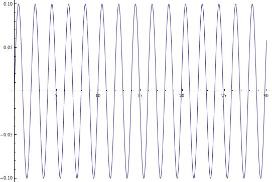
where m indicates an index of refraction, $\psi_n$ and $\zeta_n$ (and their respective primes) are the Ricati-Bessel functions chosen, and $\alpha$ and $\beta$ are constants given by wave parameters (k, etc). These scattering coefficients are then combined with a mathematical tool called a “Legendre polynomial” to give amplitude functions for the scattering. Other parameters can then be derived once these functions are modeled.

Tools

Mathematica
LaTeX

Timeline

Week 1 (4/7 – 4/13)

I will refresh and further extend my knowledge of Mathematica and continue my research into the computational and theoretical aspects of Mie scattering in the context of the interstellar medium (ISM). As my project is computationally based, I will focus heavily on bridging the divide between my theoretical knowledge of scattering in the ISM and my work in Mathematica.

Week 2 (4/14 – 4/20)

For Week 2 I plan on completing a working Mathematica model for the asymmetry parameter, g, and complimenting this work as needed with research into Bessel and Ricati-Bessel functions. Mie theory is founded in the rigors of these functions and gives solutions to Maxwell’s equations that illustrates the scattering of waves by spherical particles. Specifically useful with the Bessel and Ricati-Bessel functions are the eponymous differential equations. If this work is completed I will move on to Week 3 work.

Week 3 (4/21 – 4/27)

I will continue modeling. My initial research into the theory will be added to as needed. As time permits, I will continue on to explore the utility of Mie theory and scattering within the ISM as it relates to the derivation of other interstellar grain properties.

Week 4 (4/28 -5/4)

I will finalize any lingering modeling. My results will be nearly all in and I will begin to wrap up my blog – focusing on visualizations (plots and animations) and ensuring that they function properly within the blog space. This week will be mainly devoted to polishing off my blog posts (data and results especially), i.e. making all aspects of the blog look aesthetically pleasing.

Week 5 (5/5 – 5/11)

This week concludes my project as I finish commenting on my peer’s blog posts.

Collaborators

While I plan on working alone, Professor Magnes will be assisting and advising as this project progresses. Both of my predecessors focused on the theory and modeling of Rayleigh scattering – a related phenomena but still outside of the purview of my project. I intend to move in a direction much different than my predecessors who explored scattering of the Rayleigh domain. I do, however, anticipate that as my project develops, I will be reflecting on my results and the possibility exists to compare and contrast them in the context of the work done by these individuals. I cannot predict what these comparisons may entail, but as I conclude my project, these ties may reflect elements shared between background theory, computational processes, and my results.

Project Plan: RLC Circuits

Plan/Goals:

In this project, I plan to study the relevant differential equations that govern RLC circuits and use Mathematica to solve them for values that are useful. The general equation governing a basic RLC circuit with a capacitor, voltage, resistor, and inductor in series, in that order is:

$LI'(t)+RI(t)+\frac{1}{C}Q(t)=V(t)$ [Equation 1] (UBC- Source 4)

which, when going through a series of substitutions, becomes:

$LI''(t)+RI'(t)+\frac{1}{C}I(t)=\omega E_{0}cos(\omega t)$ [Equation 2] (UBC- Source 4)

Equation 1 has six variables: L (inductance), R (resistance), C (capacitance), V (voltage), Q (charge), and I (current). When a circuit like this is set up in the lab, the values that are known are L, R, C, and V because they directly depend on the components of the circuit. Once the differential equation [2] is solved, values for current (I) and charge (Q) can be determined. I will use Mathematica to solve for the general solution to this differential equation [2], which is a second-order differential equation. Once I have the general solution, I will vary the initial conditions to determine the effect of different circuit components on the overall properties of the circuit. Following this, I will develop more series RLC circuits with components that are set up differently in terms of their component structure.

Timeline (Weeks 1-5):

Week 1: I will begin by reviewing basic differential equation solving techniques for first and second order differential equations. I will also study the differential equation solving capabilities of Mathematica and review the techniques for solving second-order differential equations as they apply to RLC circuits.

Week 2: I plan on solving for the general solution to Equation 2 above (using Mathematica). I will vary different initial conditions and create graphs that visualize the changes that occur. I will also have a visual representation of the circuit.

Week 3: Develop another series circuit or study a previously built one. Determine the general equation for it and begin the solution process.

Week 4: Finalize the solution for the second circuit. Develop graphs for visualization purposes.

Week 5: I will finalize my project by proofreading all the components and making sure everything is presentable. I will also provide constructive criticism to my peers on their projects.

Sources:

1. Mathematica Cookbook by Sal Mangano

2. Electronic Circuit Analysis for Scientists by James A. McCray and Thomas A. Cahill

3. Dynamical Systems with Applications using Mathematica by Stephen Lynch

4. The RLC Circuit- University of British Columbia- http://www.math.ubc.ca/~feldman/m121/RLC.pdf

5. Class Notes- Mathematics 228 (Methods of Applied Mathematics) taught by Matthew Miller

Collaborators:

N/A

Project Proposal – Scattering and the Interstellar Medium (ISM)

For my project, I will be studying Mie scattering and it’s relevance to the study of the interstellar medium. The ISM, the space between stars and galaxies, is filled with gas (atomic and molecular), dust, and is permeated by radiation – starlight. Observations of various astrophysical phenomena show that along a given line of sight, their is “extinction” of this radiation. Scattering and absorption account for these observations and occur due to the presence of various dust grains within the ISM. I will model Mie scattering and look at the asymmetry parameter g, a measure of the fraction of light scattered in the forward direction, in an effort to model the relationship between this value and dust grain properties such as size, composition, etc.

Project Proposal: Diffraction Symmetries of C. elegans

The C. elegans nematode is a common subject of biological studies, and has become more and more popular in physics research. I intend to find the diffraction patterns generated by the worms’ shape and log the findings into a Symmetries Library (with the eventual goal of using Group Theory to get the worm shape directly from a diffraction image).

The shape of the worm (photos to be taken with a microscope) will correspond to a particular diffraction pattern. I will model the Fraunhoufer diffraction patterns (Far-Field diffraction) of the electromagnetic waves (light waves) by generating images with Mathematica using the Fourier Transforms. The idea is that $\left | Fourier Transform | \right ^2 $ = the diffraction pattern. This project is a study of the behaviors of light waves.

I will eventually be keeping a log of my findings on the already existing website, the Diffraction Symmetries Library.

Developing Models of RLC Circuits

For my project, I will study RLC circuits. RLC circuits have three main components; resistors, inductors, and capacitors. These circuits are important because of their prevalence in radios and televison (among other things). Specifically, I will develop a few different configurations of these circuits and measure characteristics such as voltage, current, resonance, and most importantly, damping. The physics that governs RLC circuits relies heavily on the mathematics of differential equations. For this reason, Mathematica, due to its strong capabilities in regards to differential equations, is the ideal program to use to model and study these systems.

Modeling and Experimental Tools with Prof. Magnes

Ideal for getting ideas and feedback on upper level physics tools.