Category Archives: Fall 2016

Computational Physics Projects Fall 2016

Viscous Drag and Motion

Overview

This project aimed to simulate the viscous drag forces that occur when a ball falls in fluids with different densities and viscosities, resulting in different Reynolds numbers. In this case, there are two graphs produced. The first shows the ball falling in the medium in phase-space. The second shows the vertical distance traveled by the ball in time. The ball falling in the fluid with the larger Reynold number should take a longer time to fall because the drag forces on the ball are greater. Fluids include both liquids and gases.

Reynolds numbers determine the type of flow the fluid will make. When Re<<1 the fluid follows Stoke’s Law. When Re>>1 the fluid does not,it follows the Navier-Stokes equations. The Reynolds number is a proportion of the inertial forces to the viscous forces, Re = inertial/viscous.

Motivations

While I studied abroad, I took a fluid dynamics class that covered the Navier-Stokes equations and complicated geometries of objects moving in fluids. The most basic geometry is a sphere in 3D and a circle/disk in 2D. I wanted to be able to visualize and create a code that could interpret various inputs for fluids and produce a 2D plot of the motion. It proved more difficult to do than initially thought because I do not have a solid background in fluid dynamics, just that one course. As a result, I referenced derivations for the Navier-Stokes, but most were more complicated than the 2D system I wanted to model. I referenced my notes from the course too and YouTube videos from MIT.

Figures (click on the images to make them larger)

Figure 1. The parameters of this plot are those of water and honey at room temperature (20° C). The viscosities are 1.0 (Pa s) and 1.36 (Pa s) and the densities are 0.7978 (kg/L) and 7.20 (kg/L) respectively. The ball travels slower in the honey, Re2.

Figure 2. The parameters for this plot are viscosities of 32 (Pa s) and 400 (Pa s), densities of 20 (kg/L) and 75 (kg/L), and kinematic viscosities of 1.6 and 5.33, respectively. The Reynolds numbers are displayed on the plots. The ball moves slower in the larger Reynolds number fluid.

Fluid Mechanics Physics

The above equations are the Navier-Stokes equations in 3D for cartesian coordinates. For the 2D version that I used, the z-direction components are removed. These equations are only used for when Re>>1, for high Reynolds numbers. Because the Navier-Stokes equations can only be solved for very specific cases I simplified the process by using the drag equation,

and then solved Newton’s second law for the vertical and horizontal directions, and formulated the kinematics equations. Buoyancy forces were ignored. This is a different case than than when Re<<1.

When Re<<1, the system follows viscous drag using Stoke’s Law

From here you can solve Newton’s second law and formulate the kinematic equations again. Stoke’s Law only works for these cases, otherwise Navier-Stokes and the drag equation are used. Buoyancy forces were ignored here too.

Results

Computational fluid dynamics (CFD) is a growing and complicated field of both mathematics and physics. The program I developed is part of the general sphere of CFD but not close to the type of programs are used and developed. CFD is used to simulate airplane designs, model the way fluids flow around objects. My program has some bugs because of the simplifications I used for the equations. By using an adapted version of the Navier-Stokes equations, not all parameter values work correctly with the model. For the many combinations of inputs, however, the larger Reynolds number fluid produces a slower movement in the fluid.

Conclusion

In the future, I would like to fix the bugs caused by the simplifications and possibly create a program that uses the Navier-Stokes equation in its full 3D form. If possible, it would be useful to have a GUI for the program because that would allow the user to more easily see the differences in the motion when the viscosities and densities of the fluids are changed. Perhaps adding more than two fluids to the model as well as making the visualization as a movie and not stagnant plots.

References

http://soliton.ae.gatech.edu/labs/windtunl/classes/hispd/hispd06/ns_eqns.html

http://www.personal.psu.edu/wzl113/Lesson%20Plan.htm#GF

http://scienceworld.wolfram.com/physics/StokesVelocity.html

https://www.grc.nasa.gov/www/k-12/airplane/nseqs.html

https://www.grc.nasa.gov/www/k-12/airplane/reynolds.html

Analysis of C. Elegans Worm Diffraction Patterns using Lag, Density, and Poincaré plots

Overview & Background:

For my project, I analyzed non-saturated data taken in Professor Jenny Magnes’ laboratory of “roller” and “wildtype” C. elegans. worms. The goal was to use computational techniques to differentiate between worm types. To this end, I created three different types of graphs: lag, density, and Poincaré plots. All three used normalized data. Although my lag and Poincaré plot codes create 2D plots comparing non-lagged to lagged data as well as 3D plots that compare multiple lags, I am only including the 2D plots here due to the number of graphs I have.

Lag plots display the value of the data at time (t) versus the data at time (t – lag), where lag is a fixed time displacement. These plots determine whether data is random or not. They are one method for inferring information about dynamical attractors from observations.[1] The time delay is used to reconstruct the attractor. I plotted lag plots with lags of 200 and 400 (Figs. 1-2).

I then created density plots by binning the data into a 50 x 50 matrix and plotting the intensities of values in each bin (Fig. 3). These plots give information about the number of times point (x,y) appears in each plot by representing the counts with color. The density plot code also calculates the area of each plot divided by the area of values equal to zero (AreaRatio) and the area of each plot not equal to zero over the area of values that are (zeroRatio) (Fig. 5). These ratios describe the motion of the worms, specifically how much area they use to move around in.

Finally, I created Poincaré plots by plotting each value (point at t) against the next chosen value (point at t + lag) (See Fig. 4). Poincaré plots are return maps that can be used to help analyze data graphically. The shape of the plot describes how the system evolves over time and allows scientists to visualize the variability of their data.[2] They have two basic descriptors: SD1 and SD2.[3] Defining the “line of identity” as a 45-degree diagonal line across the plot, SD1 measures the dispersion of points perpendicular to the line of identity while SD2 measures the dispersion of points along the line. My code calculates and returns these statistical measures as well as the ratio SD1/SD2 for each lag determined by user input. For this project, I used lags of 1 and 100 (Fig. 6).

Results:

I. Lag Plots

Fig. 1 Lag plots of Roller Worms 3.20, 3.26, and 3.34 for lag values of 100, 200, and 400.

Fig. 2 Lag plots of Wildtype Worms 18, 19, and 26 for lag values of 100, 200, and 400.

II. Density Plots

Fig. 3 Density Plots of Roller worms 3.20, 3.26, and 3.34 (left) compared to Wildtype Worms 18, 19, and 26 (right) with lag 200

III. Poincaré Plots

Fig. 4 Poincaré Plots of Roller Worms 3.20, 3.26, and 3.34 (top) and Wildtype Worms 18, 19, and 26 (bottom) for lag values of 1 and 100

IV. Data

Fig. 5 Values of SD1, SD2, Ratio of SD1/SD2, Area Ratios, and Zero Ratios for Roller Worms 3.20,3.26, 3.32 (left) and WildType Worms 18, 19, and 26 (right) for lag values of 100, 200, and 400 as well as average values per worm-type (bottom).

Discussion:

The lag plots indicate that my data is non-chaotic because they all had non-random structures. There appears to also be differences between worm-types, although this difference is difficult to quantize. As the lag increases, the lag plots appear more chaotic for both worm-types, moving from aligning with the x = y line to appearing more random and diffused. The plots show a difference between worm-types, but quantifying this difference will take further analysis. Wildtype worms tended to fall closer to the x = y line than roller worms. This is a sign of moderate autocorrelation. This suggests prediction of future behavior is possible using an autoregressive model.[4]

The density plots show a clear distinction between worm-type, with rollers tending to have more circular-shaped plots with highest intensity values at the center while wildtype worms appear to take up less of the plot area, with highest intensity values along the diagonal and at the center of the plot. This is confirmed by the area and zero ratios (Fig. 5). Wildtype ratios were on average larger than those of rollers, with area ratio values ranging from 0.04-0.4 more and zero ratio values ranging from 0.1-0.4 more for rollers. This gives us a quantifiable way to measure the difference between the motions of the two worm-types. However, whether these differences are statistically significant or not remains to be seen.

The Poincaré plots show little difference from the x = y line for a lag of one. However, at lag 100 they do deviate from the line. Although lag differences between the worm types are difficult to quantify, these plots do appear to follow similar patterns to those in the previous two types of plots. The values of SD1 and SD2 helped quantify plot differences. Although SD1 did not differ on average by a notable amount (~0.0008-0.1), SD2 did show a notable difference. For the average roller, SD1 was approximately 0.3 for all lags. SD2 for wildtypes was around 0.5. The SD values decreased as the lag increased for both worms. These values resulted in a SD1/SD2 ratio for rollers over 1.3 times larger than that of the wildtype for all lags.

Conclusion & Future Steps:

These results indicate it may be possible to discern between worm-types using the computational methods described above. However, further analysis of the plots as well as analysis of more worm data is necessary to draw definitive conclusions. Statistical analysis should be employed on the ratios and SD values listed in Fig. 5 to determine whether they are statistically significant. This code could be used in the future to check if data is random or chaotic, find patterns in data, and compare and differentiate data sets. Certain improvements could be made to the code. The Poincaré code could plot the ellipse with SD1 and SD2 as shown in source [3]. The density plot takes longer to calculate at higher bin numbers, which corresponds to higher resolution. Improvements could be made to the code to improve computational time. This code also can only run one lag at a time. With improved speed, it could be altered so users can input as many lags as they want at a time, like with the Poincaré and lag plot codes.

References:

[1] Sauer, Timothy D. “Attractor Reconstruction.” Scholarpedia. 2011. Web. 11 Dec. 2016. <http://www.scholarpedia.org/article/Attractor_reconstruction>

[2]Golińska, Agnieszka K. Poincaré Plots in Analysis of Selected Biomedical Signals.” Studies in Logic, Grammar and Rhetoric. 2013. Web. 11 Dec. 2016. <https://www.degruyter.com/view/j/slgr.2013.35.issue-1/slgr-2013-0031/slgr-2013-0031.xml>

[3]Goshvarpour, Atefeh. Goshvarpour, Ateke. Rahat, Saeed. “Analysis of lagged Poincaré plots in heart rate signals during meditation.” Digital Signal Processing. 2015. Web. 11 Dec. 2016. <https://www.researchgate.net/publication/222569888_Analysis_of_lagged_Poincare_plots_in_heart_rate_signals_during_meditation>

[4] “Lag Plot: Moderate Autocorrelation.” NIST SEMATECH: Engineering Statistics Handbook. Web. 11 Dec. 2016. <http://www.itl.nist.gov/div898/handbook/eda/section3/lagplot2.htm>

Overview:

For my project, I created a 3 dimensional “random walk” and oriented it to be inside Minkowski’s spacetime light cone. In this case, since this is a physical interpretation of spacetime, the random walk was only in 2 directions (the x and y axis) and the iterated up through spacetime (the ct axis). The bottom (red cone) symbolized the past and the choices and movements up until the present (the intersection between the bottom cone and the top cone), which leads to the present, and all the possible paths that could be taken, as modeled by the random walks. Although it is a random walk and shouldn’t travel too far from the starting point, except in the ct direction, since the Minkowski light cone is the region of spacetime that can be travelled according to the speed of light, the walk must never move faster than the speed of light. That is, the random walk must never enter the space outside the cone, called Elsewhere by Minkowski.

My motivation for this project was to simulate an accurate model of motion through space time that could be used for education purposes. Spacetime is often viewed as a complex perspective of the nature world and a simulation would most likely help students understand the concepts such as elsewhere and the limits of the cone. In this simulation, the parameters of the random walk can be altered so the walk could travel in one direction until it dies, but the walk will never be able to leave the cone. This follows the laws of general relativity and can help students better understand relativity and its assumptions.

General Physics:

The general physics behind the random walk is having an equal probability of the walk’s next step to be in either the positive or negative direction for each direction (x and y).Then the constraints of a cone are applied to the walk so that the walk can never reach and surpass the boundary of the cone. However, if specific cases of this walk are analyzed, such as the case when the walk always moves in the positive direction for say the x direction, the walk can actually slip through the boundaries of the cone. This is because the walk’s symmetry, which will look like a square, does not match up with the cone’s, which is circular.

A solution to this is to get rid of this step iteration in cartesian coordinates. By changing the randomness from a two dimensional (x and y) system, we can actually change it to a one dimensional system and use polar coordinates. That way the symmetries will both be circular and there won’t be any inconsistencies between the walk and the cone.

Visualizations:

In the programming, the simulation would include a few different examples of which paths the random walks could take over a time of 100 iterations. Each walk was colored coded so that it could be distinguished from the others. While the simulation ran at a slow pace, so the observer could see the simulation run, the figure slowly rotated along the x and y direction so that the observer could truly distinguish between the walks. Also on the figure were short explanations of what each region of the figure was and confusing terms has a short physical interpretation.

untitled

In figure 1. We see the figure produced by the random walk code in 3 dimensions, with a random motion in the x and y directions, but the code actually using polar coordinates, and the ct direction, spacetime. Small text boxes are added to the figure to provide a short description to help better explain Minkowski’s spacetime light cone.

finaldraft

In figure 2. We see a basic image of the random walk in 3 dimensions. However this walk uses a cartesian coordinate system.

Discussion:

Throughout the process and project, I created a random walk that was confined into a cone. I am pleased with the way the code and program turned out and the computational knowledge that I learned. These walks both used the simple cartesian random walk as described by Giordano as well as one utilizing a polar coordinate system. I do believe that some additional work could be done on this project. That work includes a past random walk that leads to the present. Another interesting future project is the continuous update of the cone with each iteration of the random walks. The cone would shrink with each step as the choices the walk could take also shrink. Something else worth considering would be the relativistic effects that would occur to the particle and the walk as the particle nears the speed of light, and the boundary of the cone.

References:

Giordano, Nicholas J., and Hisao Nakanishi. Computational Physics. 2nd ed. Upper Saddle River, NJ: Prentice Hall, 2006. Print.

Simulation of a Squash Ball

The data generated in my project consisted of position data for the path of a squash ball in motion in the spatial context of a squash court. Additional important generated data included the velocity of the ball (in 3-dimensions) at any given time. Euler’s method was a relatively practical numerical method, as it made calculating the position at each step of dt (which was imperative in the animation aspect of the project) a simple matter of using the position and velocity information from the previous time step.

Some difficulty arose in attempting to achieve a smooth animation, due partly to computational time. Ultimately the solution for animating the path of the squash balls necessitated creating matrices for the position of the ball in each dimension in Cartesian coordinates. After this, the comet3 function was used to animate the plot, as it the head of the comet nicely approximated the shape of a ball, and the tail was very useful in showing the entire path of the ball from its initial position.

In the end, my goals for the project had to be altered slightly, as attaining the user-friendly inputs that I had wanted proved to be a complicated task. I had initially hoped that the finished product would allow for a user to input some initial velocity using the arrow keys. Ideally the user would hold down some combination of the arrow keys for some amount of time, and then press the spacebar to initialize the loop and set the ball in motion. Based on the amount of time each direction arrow had been pressed, the ball would be imparted with a corresponding initial velocity. However, unfortunately Matlab’s capabilities to not allow for the reading of key presses without the use of user-generated GUI’s. Given that my understanding remains relatively basic, I had to scrap my dreams of user-interaction with the model.

Though the ultimate goal of my script was an educational experience for the user, writing the script was a learning experience in itself. I had previously modeled some colliding pendulums in Matlab, and I drew on this code in scripting the ball-to-wall collisions, and subsequently the resultant velocities of the ball was an easy task. In the early draft of my code I encountered some problems, as certain initial velocities seemed to result in the ball getting stuck inside the walls – an obviously undesirable result due to its physical improbability. Having encountered a similar issue in my colliding pendulums code, I knew that the problem had something to do with the script not checking on the position of the ball often enough, due to the time step, ‘dt’, being too large. While this was part of the problem, the larger source of the issue was the fact that, once beyond the wall, the ball’s velocity was rapidly decreasing, as the script believed that it was continuously colliding with the wall. In the end the fix was relatively simple: if the ball passes beyond the wall, reset the balls position so that it is at the wall again. Though simplistic, this is a powerful idea in the context of computational methods. If having a variable reach a target value is desirable for your simulation or simplifies the problem, just check that the variable comes within a reasonable range and set it to the target value.

I was surprised to note how relatively close to the front and right wall many of the balls ended up. This was most likely due to the fact that my expectations came from having played squash. When returning the serve, the goal is to hit the ball back before it bounces twice, therefore if you have watched to ball until it stops rolling (as the script does), you have long since lost the point. It was interesting to confirm that the majority of serves bounce twice within the confines of the larger box in the back left of the court (makes up about a quarter of the floor) which verified my own experience that almost all serves are returned from the back left of the court. Though these results seem quite inconsequential, the objective of the script is an educational experience, so these observations can be read as positive outcomes.

The goal of my script was entirely focused on user experience. Consequently, the product of the script was not heavy on calculated results. The main idea was for users to be able to gain an intuition for the flight path of a squash serve without ever having played, or even seen the sport being played before. On the other hand, it may have been interesting to take the project in a more numerical-result-driven direction. For instance, a comparison of the initial angle of the ball with the final angle would have made for an interesting discussion. Having run through the script a number of times, and therefore seen at least a hundred individual ball paths fully plotted, a distinction between the serves that struck the side-wall before the back-wall, and those that did the opposite definitely emerged. Quantifying this difference could potentially be illuminating. Another question that might be considered concerns the balls that hit the side-wall and back-wall simultaneously. How would these corner cases (pun intended) show up in the data? If I were to modify the script to accomplish this, the most important change would be to increase the number of iterations from ten into the hundreds or even thousands. This would almost certainly necessitate abandoning the full animation of the flight path, and focusing instead on the location of the ball’s second bounce on the floor (when, according to the rules of squash, the point has ended).

If I were to instead expand my project to expand the user’s experience and fully embrace the educational aspect of the project, I would certainly want to solve the problem of more interactive user input. Allowing the user to control the velocity would allow them to develop a feel for the serve without ever having stepped on a court, whereas the project in its current state relegates the user to the role of an observer, rather than an active participant. Ideally the project could be taken beyond the confines of a serve, and allow the user to control a player that plays out a full point, perhaps against a computer-controlled player. This would potentially require quite complex user input capabilities (for position of the player and velocity and direction of each hit) and would also necessitate a method of plotting that was instantaneous. A more simplistic full-point simulation could also be created by creating additional collision areas that represent swinging rackets at various locations the court, so that a ball that happened to reach that position would be imparted with some new velocity and direction.

Sources:

<http://www.worldsquash.org/ws/resources/court-construction>

<http://www.worldsquash.org/ws/resources/rackets-balls/racket-ball-specifications>

Atomic Diffusion

The project focuses on creating a visual model displaying the random movement of an atom through various structures. The program models and compares the substitutional diffusion of atoms through a two-dimensional fractal and three three-dimensional types of crystal lattices. The models created are most useful in visually understanding the process of diffusion and the impact of the structure in determining the process of diffusion. These could be used in any class that discusses basic crystallography and solid state physics to help visualize the processes within the structures.

Background:

Atomic diffusion is the random thermal movement of atoms through a solid. In crystals, atomic diffusion can occur through interstitial or substitutional means. Interstitial diffusion refers to when atoms move in between the lattice points of a crystal. The atoms have a slightly greater freedom of movement, as the only conditions are that there is an unoccupied location adjacent to the particle and that the particle has enough thermal energy to diffuse there. Substitutional diffusion, which is the focus of this project, occurs when an atom takes the place of an atom in the lattice. The atom can thus move around the lattice by switching places with other atoms.

Crystal lattices are the periodic repetition of a structure, where the base unit is known as a unit cell. The unit cell of a lattice can be determined based on the locations of the fewest lattice points needed to repeat the structure. Thus, for a simple cubic lattice, with one lattice point at each edge of a cube, the lattice can be described by the point at (0,0,0). With repetition, this point repeated in each direction every length a (the lattice constant) will create a simple cubic lattice. A body-centered cubic lattice is a simple cubic lattice with an extra lattice point in the center of the cube. It can be described by the two points (0,0,0) and (1/2,1/2,1/2). In comparison, a diamond lattice is more complicated. Found commonly in diamond itself and in semiconductors such as silicon, a diamond cubic lattice requires eight lattice points to repeat the structure. These points are located at (0,0,0), (0,1/2,1/2), (1/2,0,1/2), (1/2,1/2,0), (3/4,3/4,3/4), (3/4,1/4,1/4), (1/4,3/4,1/4), (1/4,1/4,3/4).

Model:

The program is separated into two sections. The first section creates a fractal by plotting the real and complex parts of the solutions to an iterated complex equation against each other. Several particles are placed inside the fractal and consecutively allowed to randomly walk in two dimensions. The fractal acts as a wall for the particle’s movement. The program limits the particle’s movement by either stopping the particle from moving within a certain radius of the fractal’s edge, or by resetting the particle to the origin. The particle’s motion is plotted and tracked for clarity of understanding the motion of the particle. The section demonstrates diffusion by random walk in a large section of a medium, limited by boundaries.

The second section of the program plots a simple cubic lattice, a body-centered cubic lattice, and a diamond cubic lattice. A particle is placed at the origin of each plot and allowed to move randomly to adjacent lattice points. The lattice constant is set to be four, and each particle can move a distance of at most magnitude five per time step. This allows the particle to move to any nearby point via substitutional diffusion. The particles’ movement is plotted for their first 200 steps.

Several key assumptions are made by the program. First and foremost, all adjacent points are considered equally likely locations for the particle to diffuse to. This assumes that all directions and distances up to a distance magnitude 5 away are equally viable for the particle’s movement, and that the particle does not lose energy over the course of diffusion. It also assumes that all atoms in the lattice, apart from the additional particle (shown in red) are the same element, isotope, and chemical properties. Secondly, it is assumed that the new atom can easily displace the previous atoms. These assumptions allow the program to easily model the movement of the atom for visualization purposes.

Data:

$fractal-diff$ $fractal-diff2$

Figures 1(a) and (b): 2D diffusion of particles on a fractal.

The above figures represent two iterations of 2D diffusion on a fractal. The fractal is plotted in red, while the movement of the particles are plotted with one dot corresponding to one step taken by a particle. The figures show the range of the motion of the particles. While the program generally confines the particle to the interior of the fractal, as can be seen in both figures the particles can be capable of diffusing past the fractal’s boundary. Diffusion across a boundary can occur when there is a lower activation energy for diffusion and when there is a defect or open lattice point on the other side of the boundary.

Figures 2(a), (b) and (c): 3D diffusion on various crystal lattices.

The particles diffuse through the lattices as intended. The particle in the simple cubic lattice travels farther, while the particle in the body-centered cubic lattice remains slightly more compact in its diffusion. This follows from the probability of motion and the assumptions that were made in the program. As a body-centered cubic lattice has more lattice points close to the original, there is a slightly higher probability that the particle will remain close to the original location. This effect is small, as the particle has only one additional lattice point per unit cell that it can reach. Similarly, the path of the particle in the diamond cubic lattice displays compactness close to the origin. As before, this is due to a small increase in the probability that the random motion of the particle will go to a nearby lattice point, as there are significantly more lattice points per unit cell in the diamond crystal lattice than in the simple cubic or body centered cubic lattices.

The model is perhaps most effective in its ability to rotate or to be moved in three dimensions while the particle is diffusing. The model can also display the diffusion in each of the two-dimensional views. The ability to manipulate the view of these diffusions allow a greater understanding and intuition of lattices and the motion of particles within lattices.

The model does not consider multiple particles diffusing at once, more complex atomic alignments within the lattice, or diffusion methods other than substitutional. The program also struggles to effectively model large crystal structures, as such structures use substantial amounts of memory. However, for smaller scale models or for varying time scales, the program and its models are very effective.

Conclusion

The program effectively plots three-dimensional random substitutional diffusion on three lattice structures. It similarly plots two-dimensional random diffusion on a fractal structure. The fractal confines most particles to within its bounds and explanations are offered of cases where diffusion can be seen to cross boundaries. The four models can be used as educational tools, increasing knowledge and intuition for students about diffusion in solid-state systems.

Sources

[1] Giordano, Nicholas J. Computational Physics. Upper Saddle River, NJ: Prentice Hall, 1997. Print.

[2] Kittel, Charles. Introduction to Solid State Physics. New York: Wiley, 1986. Print.

[3] Shaw, D. Atomic Diffusion in Semiconductors. London: Plenum, 1973. Google Books. Web.

Multi-component Dynamics of Particles from Nonequilibrium

Background and Motivation:

Many ordered physical phenomena such as ferromagnetic materials and solid state crystals are formed in nature from a nonequilibrium state of many particles or components, often with various distinct types or properties. Though studying single particle or two particle systems are essential to understanding physical phenomena at fundamental scales, the complex systems presented by multicomponent, many particle systems present interesting problems, and may come with significant practical applications. For example, ferromagnetism is a widely used and familiar phenomenon involving a large number of particles in an ordered solid. In the first half of the 20^th century, physicist Ernst Ising was able to provide a mathematical model for magnetism by employing a simple dynamic two-component system of discrete particles in a lattice. Magnetism arises as an inherently quantum mechanical phenomenon that can be described as a collection of atoms with non-zero electron spin states and their associated magnetic dipole moments. The Ising model uses statistical mechanics and simplifies the system to a graph of particles with two possible states, spin up or spin down, interacting according to nearest neighbor approximations. Though the model is a gross simplification of the physical system, it is actually able to predict phase transitions across a temperature threshold from, say, ferromagnetic states to nonmagnetic states. Furthermore, due to the discrete nature of the model, it can smoothly be implemented in computational simulations without much loss of generality. An implementation of the Ising model in MatLAB, and mapping the associated phase transition, is described below.

Models involving multiple-component dynamics from nonequilibrium states can also be used to describe the self-assembly of molecular structures. Despite being a nonequilibrium process, self-assembly has largely been studied according to purely statistical mechanical models that consider the discrete dynamics of the particles to play no role in the evolution of the system except to convey the concept that systems tend to evolve along paths that minimize the free energy of the system [2]. Though this assumption holds for systems in near equilibrium states or for simple systems under mild nonequilibrium conditions, descriptions that do not account for the dynamics that emerge out of local interactions between particles fail to accurately describe the evolution of systems far from equilibrium. This is particularly true for self-assembly processes that reach thermodynamic equilibrium on long time scales with respect to experimental or computational limitations. For example, a system of particles forced into harsh nonequilibrium conditions, such as a liquid that is rapidly supercooled, may experience binding errors during crystallization, leading to kinetically trapped structures corresponding to “randomly” emergent local minima on the free-energy landscape. It is worth noting that kinetic trapping can also affect self-assembly of multi-component solid state systems under mild nonequilibrium conditions due to the slow mixing of components within a given system.

The Ising Model:

The Ising model was originally developed by German physicists Wilhelm Lenz and Ernst Ising in the 1920s. As stated above, the Ising model simplifies a magnetic solid by assuming that particles are fixed to an evenly spaced lattice of points and all have spin states aligned in either the +z or –z direction ( ${$ s = +1$}$ or ${$-1$}$ ). Due to interactions between nearby magnetic dipoles, particles have particular energy states associated with them according to a nearest-neighbors approximation. Here, a two-dimensional Ising model is implemented with each particle having four nearest-neighbors, as shown in Figure 1. The interaction energy between two particles with parallel spin components is given by ${$\epsilon_s$}$ (the subscript ${$s$}$ denoting “same”), and the interaction energy between two particles with antiparallel spin components is given by $[$\epsilon_d$$ ( ${$d$}$ denoting “different”). According to the theory of magnetism, magnetic dipoles with parallel alignments are in lower energy states than those with antiparallel alignments. This condition is satisfied by ${$\epsilon_s - \epsilon_d > 0$}$ .

isingmodelfigure

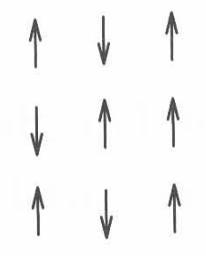
Figure 1. Schematic spin model for a ferromagnet. [1]

The dynamics of the model is achieved by randomly choosing particles at some rate ${$c$}$ to flip to its opposite spin state with a success rate proportional to a Boltzmann factor with respect to the energy of the chosen particle. This probability is given by given by ${$min( e^{-\Delta E/k_B T},1) $}$ , where ${$\Delta E = \left( \sum_{<i,j>} \epsilon_{<i,j>} s_{i,j,flipped} s_{<i,j>} \right) - \left(\sum_{<i,j>} \epsilon_{<i,j>} s_{i,j,current} s_{<i,j>} \right) $}$ and ${$<i,j>$}$ indexes over all four nearest neighbors. It becomes apparent that for flip events with ${$\Delta E < 0$}$ flip with a probability of unity, corresponding to a lowering of energy, and that there is also non-zero probability for a particle to flip to a higher energy state [1]. However, the system should tend toward microstates with lower energy on a statistical whole, eventually approaching some minimum value given a finite number of particles and space.

Results and Analysis:

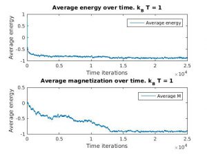
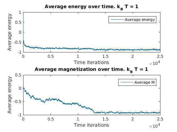
Figure 2(a) and 1(b): Monte Carlo implementation of Ising model (2D). Figure 2(a) shows a time series plot of the spin lattice. Lattice was initiated with particles in a checkerboard pattern (ie. with alternating spins). Temperature was below critical value and no magnetic field was applied. Figure 2(b) shows plots of the average energy and magnetization over time iterations. Energy decreases over time, and magnetization tends to approach either +1 or -1, implying total parallel alignment.

As expected, the energy decreases over time, and small localized domains of aligned spins begin to appear. Total alignment (or magnetization ${$|M|=1$}$ ), is quickly approached as the free energy “reward” for parallel alignments increases. That is, at low temperatures, the Boltzmann factor is very small for positive values of ${\Delta E}$ , and thus the chance of flipping to a higher energy state is lower.

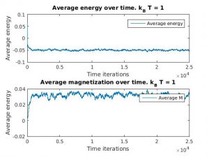
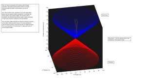
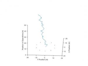
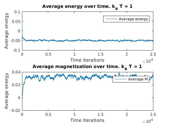
Figure 3(a) and (b): Monte Carlo implementation of Ising model (2D) with constant magnetic field in positive direction (ignore H=0 label). 3(a) shows a time series plot of spin lattice. Lattice was initiated with particles in a checkerboard pattern (ie. with alternating spins). Temperature was below critical value. Figure 3(b) plots the average energy and magnetization over time iterations. Energy approaches finite negative value and magnetization approaches finite positive value.

As a positive constant magnetic field is applied to the entire lattice, all dipoles begin to align along the direction of the magnetic field. However, once magnetized, if the magnetic field is set to zero, the magnetization will generally fall back down to zero unless the interaction energy for alignment for the material is large enough (for example, in ferromagnets).

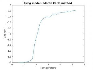
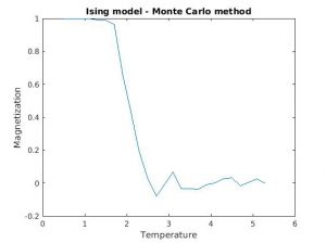
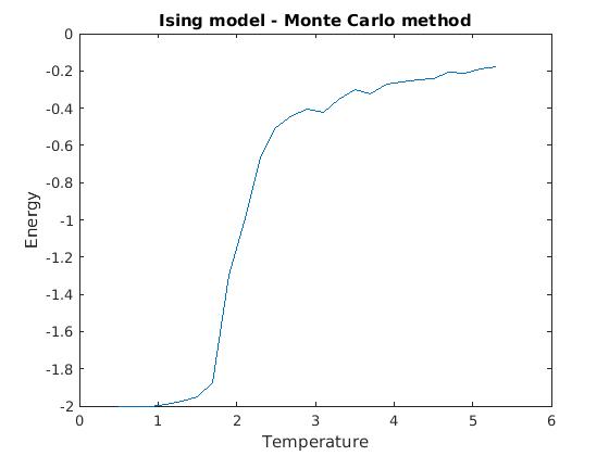
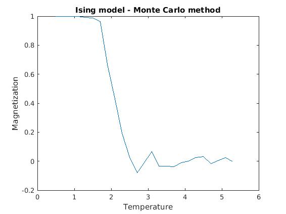
Figure 3(a) and (b): Monte Carlo implementation of Ising model (2D). Spin dynamics were calculated for each temperature value over 25,000 Monte Carlo iterations, and the last 1,000 values of energy and magnetization were averaged and plotted against temperature. All calculations were done for a 50×50 lattice, with all other relevant parameters normalized to one.

Figures 3(a) and (b) demonstrate the phase transition from a ferromagnetic state to zero magnetization. One can note some instability in both the magnetization and energy plots around 2.25 (units scaled to ${$J/k_B$}$ ), indicating a critical point in the temperature. The system becomes incredibly sensitive to small perturbations as the properties of the material are rapidly changing over temperature. Exact analyical solutions for the critical point how that ${$T_c = 2/ln(1+\sqrt{2}) \approx 2.27$}$ [1]. As T approaches 4, the system crosses the phase transition boundary according to mean field theory.

Future work:

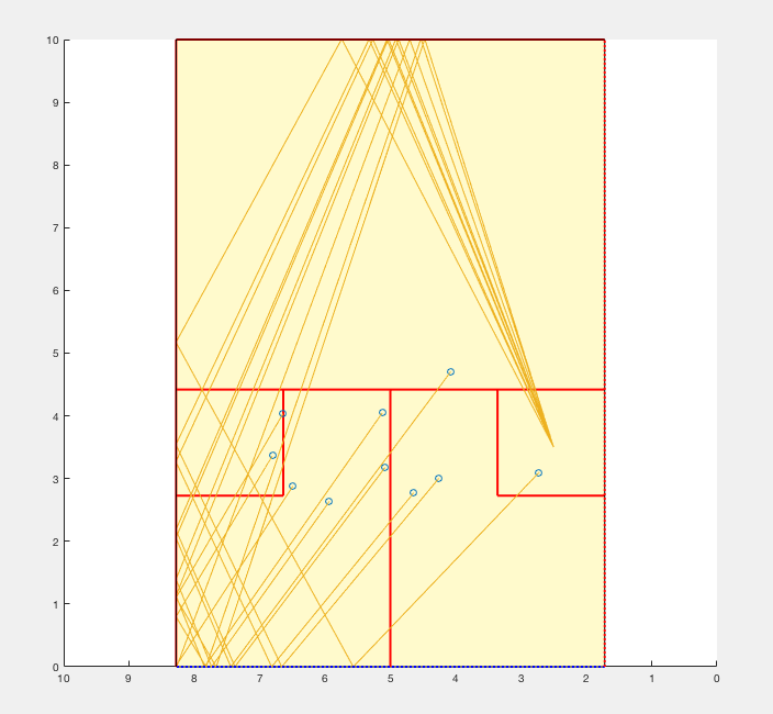
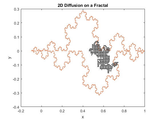
The methods utilized by the Ising model to calculate the dynamics of many-particle systems is not limited to spin systems. The assumptions made by the Ising model, such as that the system dynamics are dominated by nearest neighbor interactions between n-types of particles and obey statistical mechanics, can easily be generalized to other systems as well. For example, consider the slow deposition of molecules with two distinct conformers onto a reactive substrate surface. Supposing that there are significant intermolecular interactions between the molecules and the substrate surface and between the molecules themselves, the dynamics of the system may be simplified to a growing analog of an Ising gas with two-components forced onto an underlying lattice. If this underlying substrate has significant nonhomogenous structure on the scale of the lattice spacings, patterns in the depositing overlayer may emerge. This has actually been observed in certain organic-inorganic interfaces, and the resultant structure may play a key role in the functionality of the material [4].

Conclusion:

A Monte Carlo simulation of the Ising model was developed in MatLAB, along with some extensions to multi-component growth modeling of gaseous particles solidifying on a substrate. Ideally, my implementation of Ising model can be generalized and used to develop other multi-component simulations with more complexity. This program had a number of limitations in its practical usage and theoretical robustness. For one, the order of calculates necessary to compute various results increases rapidly with complexity. My implementation in particular was limited to simulating a 2D lattices containing somewhere between a couple hundred and a thousand points, where as magnetic solids are 3D objects containing on the order of ${10^23}$ atoms. Furthermore, though many unnecessary boundary effects were avoided by implementing toroidal boundary conditions on the lattice edges, which is useful for treating magnetism in the bulk, there is a lack of middle ground where both the bulk and the magnet edges can be accurately simulated in this model. There were also a number of significant approximations and assumptions made during the formalism of the model that affects the accuracy and relevance of the model to real physical systems. However, the model is surprisingly qualitatively powerful despite its simplicity, and has a wide range of applications to other multi-component systems.

References:

[1] Giordano, Nicholas J. Computational Physics. 2nd ed. Upper Saddle River, NJ: Prentice Hall, 2006. Print.

[2] S. Whitelam, L. O. Hedges, and J. D. Schmit, Self-Assembly at a Nonequilibrium Critical Point, Phys. Rev. Let., 112, 155504 (2014).

[3] S. Whitelam, Growth on a rough surface, 2016.

[4] C. Ruggieri, S. Rangan, R. Bartynski, E. Galoppini, Zinc(II) Tetraphenylporphyrin Adsorption on Au(111): An Interplay Between Molecular Self-Assembly and Surface Stress, J. Phys. Chem. C, 2015, 119 (11), pp 6101–6110

Gravity Assist

Overview:

The computational problem that I worked on for my final project was to simulate a satellite undergoing a gravity assist as it passes a planet. The “gravity assist” is a technique used to help spacecrafts reach targets that are “higher up” in the sun’s potential well. This program creates 2-D animations that are not centered around either the satellite or the planet to express the gravitational interactions between the two. What is meant by neither body being centered is that the both the planet and satellite are moving. The planet is used to change the satellite’s trajectory. The program itself generates a velocity graph of the gravity assist of a satellite as it passes by a planet and the velocity graph of a satellite that gets caught and temporarily orbits the planet. The program’s purpose is to show how the initial conditions of a spacecraft as it passes a planet determines its trajectory.

Methods:

The following image shows how the differential equations used in the program were derived. The equations are from a model for the earth’s orbit around a stationary sun. Assuming that the earth has a circular orbit around a stationary sun it allows for the use of constants instead of inputting information for the masses of the two bodies and the gravity between them. What was changed from the earth-sun example is that the larger body is in motion. Also instead of the “r” value being the radius from the sun the “r” value represents the distance between our planet and satellite.

The method specifically used was the Euler-Cromer method (using i+1) because it conserves energy when used with oscillatory problems. So the positions of both the planet and satellite are calculated at each time step and then the velocities are calculated accounting for how the distance between the two change. Now the velocities are based on interactions between the two bodies. In this program it is assumed the size difference between the two is great enough that the satellite doesn’t change the planet’s path.

Figures:

Figure 1: The gravity assist of a satellite as it passes nearby a planet.

Figure 2: The gravitational capture of a satellite by a planet for two revolutions.

Figure 3: Graphs of the the change in the Velocity over 5 years

Discussion:

The planet’s initial conditions were an initial position at the origin and an x-velocity of 5 AU/yr. In the gravity assist simulation the satellite began 86 AU away at (-50,-75) with an initial x-velocity of 0.15 AU/yr and y-velocity of 2 AU/yr. The program then simulated the position and velocity for 5 years and after interacting with the planet the the satellite was 4,195 AU (the “r” value) from the planet and had a final x-velocity of 0.717 AU/yr and a final y-velocity of 1.61 AU/yr. So the total velocity changed from ~2 AU/yr to ~1.75 AU/yr. The left of Figure 3 shows the change in the x-velocity over 5 years, the spike in the graph represent the satellite’s interaction with the planet and then as the two get further away the velocity settles to a constant value.

The second simulation represents a “catch and release” scenario where the satellite is caught by the planet’s gravity but as the two move the satellite is able escape the planet’s gravity. In the simulation it appears that the two touch but the figures are similar to point charges in that that the mass used for the calculations is at the very center. What seems to be the outside of the shapes is just an image representation used in the simulations.

In this scenario the planet still begins at the origin but it has an x-velocity of 1 AU/yr. The satellite now begins ~74 AU away (-55,-50), has an initial x-velocity of -0.45 AU/yr and y-velocity of 0.45 AU/yr. After 5 years and two complete revolutions the satellite is ~500 AU away (the “ODr” value) and has an x-velocity of 0.036 AU/yr and a final y -velocity of 0.157 AU/yr. The total velocity decreased from ~0.64 AU/yr to ~0.16 AU/yr, the change in the x-velocity over the 5 years is shown on the right of Figure 3.

Conclusion:

The simulations accurately modeled the gravity interactions between a satellite and a planet. If the velocities of the satellite and planet are great enough as the bodies interact (~2 AU/yr for the satellite and 5 AU/yr for the planet) then the two will pass each other with only a change in trajectory of the smaller body. But if the two are moving at low velocities that are close in value (~0.64 AU/yr for the satellite and 1 AU/yr for the planet) then the smaller body will get caught in the gravity of larger.

The “gravity assist” technique allows for fuel conservations as spacecrafts travel to higher orbits because the trajectory can be changed through interactions with planets. The drawback of the technique is the total velocity decreases after interaction with the planet, in the assist case there was a decrease in velocity by 12.5%. The limitation of the program is that it is unable to simulate changing the velocity at any point in the path which could be done with a spacecraft. Further investigations could look at finding the ideal relationships between travel time, speed, and fuel consumption when trying to reach a specific trajectory.

Resources:

Giordano, Nicholas J., and Hisao Nakanishi. Computational Physics. Upper Saddle River, NJ: Pearson/Prentice Hall, 2006. Print.

“A Gravity Assist Primer.” NASA. NASA, n.d. Web. 11 Dec. 2016.

Propagation Of A Wave Packet In An Infinite Well With Potential Barriers

Auther: Samuel Gilbert

Introduction:

This project models the propagation of a quantum wave packet in an infinite square well, and introduces between zero and three potential energy barriers. The wave packet used is a “Gaussian” wave packet (Eq. 1), and is a solution to the Schrödinger equation.

ψ(x,t=0) = C*exp[-(x-x₀)²/σ²], (Eq. 1)

C is a constant that represents the magnitude of the wave packet, x is the position variable, x₀is the initial position of the wave packet, and σ is the initial width of the wave packet.

The program is designed to be highly interactive, and therefore requests three inputs from the user – the number of potential barriers, the strength of the potential barriers, and the initial energy of the wave packet. An initial setup with three potential barriers is shown below in Fig. 1:

wave-packet-and-three-barriers

Fig. 1: Image of a sample initial setup.

The motivation for this program was to create an interactive education tool. To this end, the program provides instant feedback to changing variables such as energy of the wave packet and the strength of the barrier, which is a particularly useful tool in understanding quantum reflection, transmission, tunneling, and furthermore, the probabilistic nature of the quantum world.

Three plots are produced simultaneously – the imaginary part of the wave function, the real part of the wave function, and the probability density. In plotting the probability density, the program gives a visual representation of the fact that the position of a quantum object is not well defined, as it is governed by probability. The user will see the probability density split over a potential barrier, representing the probabilities of the wave packet being reflected or transmitted, respectively.

Methodology:

The computational method used in this program is the “leap-frog” method, as described in Giordano (1). The leap-frog method was used, because it allows for time dependence, unlike the shooting method studied in class. Our wave packet is then allowed to develop over time from the initial wave packet in Eq. 1., which it does. The leap-frog method alternates between evaluating the real and imaginary parts of the wave function. This, in essence, evaluates the wave function in ∆t/2 increments. In addition, it is notable that the time dependence of the Schrödinger equation is contained in the computational method itself, which is a beautiful way of handling time dependence. The leap-frog method can be thought of as an adapted Euler-Cromer method, as the updated real part of the wave function is then used to calculate the updated imaginary part, and so on throughout the routine. Giordano (1) cites that the leap-frog method has a numerical error of the same order as the 2nd order Runge-Kutta method. A significant portion of the code was dedicated to interactivity, and therefore deals with the presentation of the animated plots. This includes the stop button on the plots, which calls an external function which closes all windows, and also making sure the animation runs for the right amount of time.

Results:

Fig. 2 below shows three animated gifs for three different energies with one potential barrier.

1-barrier-energy-1 1-barrier-energy-2 1-barrier-energy-3

Fig. 2: One potential barrier modeled for three different energies.

These three animations represent what a user would see if the inputs were 1 potential barrier of strength 2*10^-6, and a wave packet with initial energy of 1.5*10^-33. This is just one of the many options that a user can choose. For example, the user can explore using the same initial energy, but changing the strength of the barrier. In addition, portions of the wave packet can get caught between two potential barriers, and add constructively, as shown below in Fig. 3:

trapped

Fig. 3: Wave packet caught between barriers, and constructive interference.

The wave functions can get complicated very fast by adding enough potential barriers and letting the program run long enough. These simulations therefore allow for complex systems than could be modeled by hand.

Analysis:

One of the unexpected results of this program is that the Gaussian wave packet decays over time, as shown below in Fig. 4.

decay

Fig. 4: Spreading of the Gaussian wave packet

Sawada et. al. (2) explain that a Gaussian wave packet is the sum of a few Gaussian curves. These Gaussian curves all have different momenta and velocities. Therefore over time, the Gaussian wave packet develops to show these different velocities, which is the cause of the spreading. Although a pitfall of the model used here, it works well, as this wave packet can be thought of as a superposition of quantum states decaying to the ground state. This is not what is really happening mathematically, but it does still work for the program. It can also be thought of as a formulation of the Heisenberg uncertainty principle, in that we are initially containing the wave packet to a defined space, and therefore there must be uncertainty in its momentum, which is the compositional Gaussian curves (1). Thus, it makes sense that the wave packet should spread out. Nevertheless, the spreading wave packet means that the simulation cannot run for too long without becoming meaningless – the most useful simulation comes in the beginning.

Further examination of the wave packets produced by different energies shows that the wave packets that have less energy have fewer peaks, and wave packets with large energies have many peaks. The nature of the compositional Gaussian curves is shown here, as the high energy wave packets are composed of more Gaussian curves, with each of those curves having its own energy. It is also noted that the high energy wave packets travel faster than the low energy wave packets, as expected.

Conclusion:

This program can be developed much further to include different types of potential barriers. The one used here is essentially a delta function, however it was finite in the program, as MATLAB cannot plot delta functions. However nothing prevents the program from being expanded to include step potentials and the like. There range of possible values for the strength of the potential barrier and the energy of the wave packet could also be expanded.

A natural extension to understanding the spreading of the Gaussian wave packet could be to perform Fourier transformations on the wave packet to parse out the composition of the wave packet. The spreading of the wave packet has been analyzed by Pan (3) using the “Bohmian Model.” The crucial assumption that the Bohmian model makes is that the wave packet has a definite location. This assumption, of course, contradicts Heisenberg’s uncertainty principle. However, the Bohmian model provides new inside into understanding the spreading of the Gaussian wave packet. Thus in the future, this program could potentially not only model a quantum object, but also describe mathematically and visually how the wave packet spreads out using the Bohmian model.

Bibliography:

(1) Giordano, Nicholas J. Computational Physics. Upper Saddle River, NJ: Prentice Hall, 2006. Print.

(2) Sawada, Shin-Ichi, Robert Heather, Bret Jackson, and Horia Metiu. “A Strategy for Time Dependent Quantum Mechanical Calculations Using a Gaussian Wave Packet Representation of the Wave Function.” The Journal of Chemical Physics 83.6 (1985): 3009. Web.

(3) Pan, Alok Kumar. “Understanding the Spreading of a Gaussian Wave Packet Using the Bohmian Machinery.” Pramana 74.6 (2010): 867-874. Web.

4 Body Orbital System

My model of Jupiter, Mars, and the Earth orbiting the Sun can be used as a tool for educating people about planetary motion. The planets have maintained their orbits for billions of years, but this model seeks to prove their stability and test under what conditions their orbits might become unstable. By gradually changing the mass of Jupiter, we can see that it is not until the planet’s mass is 1000 times more than its current weight that it would begin to affect the orbits of Mars and Earth. At this extremely increased mass, The Earth and Mars both exhibit unstable behavior. This model is not only interesting to those who study astronomy, but can be informative and reassuring of the Universe’s stability for those with no knowledge of the subject.

Physics and Astronomy often cause students a lot of anxiety. These subjects are not usually intuitive and can intimidate students, resulting in very few people studying the subject past high school.[1] This unfortunate occurrence must be minimized and graphical teaching tools can be an effective way to engage students. Presenting a visual representation of the often unobservable processes studied by physicians and astronomers is invaluable to a struggling student. Astronomy is inherently a visual subject and it makes sense to model computationally phenomena that may take too long to study physically. With a computational model you can map the progress of a planet for years in a matter of seconds. My model maps the orbits of Jupiter, Mars, and Earth for 20 years and includes a legend and text that makes it easily interpreted. My hope is that this model will help to illuminate the effects of planetary gravitational pull to beginning astronomy students.

Graph 1: This graph shows the orbits of Earth, Mars, and Jupiter after 20 years when Jupiter is at its normal mass.

Graph 2: The orbits after the mass of Jupiter has been increased by a factor of 1000.

These graphs are made by building equations from Kepler’s laws that make each planet sensitive to the gravity of all other planets in the system. This means that each planet will have four equations to solve for its velocity and position. The following shows the velocity equation for the x direction of the Earth.

vxE(i+1)=vxE(i)-(4*(pi^2)*xE(i).*dt)/(rE(i).^3)-4*pi^2*(J/S)*(xE(i)- xJ(i))*dt/rEJ(i)^3-4*pi^2*(M/S)*(xE(i)- xM(i))*dt/rEM(i)^3;

Each velocity equation must account for the mass and gravitational pull of the surrounding planets and can be done by manipulating Kepler’s laws. These equations should then be iterated using the Euler-Cromer Method.

The Euler Cromer Method is usually the best method to model oscillatory motion. In my first draft of this code, I modeled the lone Earth around the Sun. Because of an error in my equation, the Earth’s orbit was not elliptical. Upon doing further research, I attempted a 2nd Order Runge-Kutta model which proved too complicated to use when finishing the entire system. [2] I eventually was able to successfully use the Euler-Cromer Method which now perfectly models the orbital motion.

Conclusion:

This project was able to successfully build a teaching tool that would be really easily used in a classroom setting. The animation makes the model interesting to students and the year counter lets you know exactly when Earth and Mars would shoot off into space. While the unstable behavior only occurs under extreme circumstances, it is still an excellent lesson on the stability of the solar system. In the future, I would love to add more planets to the system, but I fear that the length of my equations and the number of matrices I would need to create would slow the computing time considerably. When I added Mars to the system, I had to create another 7 matrices and my equations increased sizably in length. In addition, the perihelion of mercury is more complicated to calculate and might pose a problem. Despite these potential issues, a system in which all 8 planets are represented would extremely enhance the model and its educational value.

Resources:

Grim, Nancy. A Force Concept Correlation Study with Instructional Methods, Anxiety, Perceptions of Difficulty and Student Background Variables. 1999. 11 Dec. 2016 <http://eric.ed.gov/?id=ED438164>.
Giordano, Nicholas J., and Hisao Nakanishi. Computational physics. Pearson Education India, 2006.

Solving Kepler’s Equation

Overview

For my final project I solved Kepler’s Equation numerically using Newton’s Method. Because it is a transcendental equation and thus cannot be used to solve for the eccentric anomaly directly, I created a program that uses iterative methods to solve it and then plots the solutions. Beyond this, I focused in particular on making the program user friendly to make it more usable as a teaching tool. For instance, I included detailed explanations of Kepler’s Equation as well as the ability for the user to change parameters. The reason I chose this project was because I wanted to deepen my own understanding of Kepler’s Equation and creating a program that teaches people about the equation helped me do that.

Program

Kepler’s Equation is as follows: M = E – e*sin(E) where M is mean anomaly, E is eccentric anomaly and e is eccentricity. The program focuses on explaining these three quantities and the roles they have in calculating orbits. The following picture (from www.jgiesen.de) depicts mean and eccentric anomaly:

In the picture, the black ellipse is the actual orbit being calculated (slightly eccentric) and the blue circle is the orbit without any eccentricity. The mean anomaly is the angle from the main body (in the solar system: the sun) to where a planet would be if its orbit were perfectly circular.The eccentric anomaly is the angle from the main body to a point above the actual orbit on a tangent circle.

The first graph that the program produces is a plot of eccentric anomaly versus mean anomaly at all values of eccentricity (0 to 1) in steps of 0.1. The shaded region represents possible values for E at fixed M or vice versa. As eccentricity is increased from 0 to 1, M and E get further apart. Next, we look at the extremes: e = 0 and e = 1:

As you can see, when e = 1, M and E are very different at most points. However, at e = 0, M and E are the same and the plot is a straight line. This makes sense looking back at the definition of M and E; an e value of 1 means that the orbit is a perfect circle and therefore the mean and eccentric anomaly are equal.

The program also allows for some interactivity so it can be used as a teaching tool; above is how the program explains the graphs of mean anomaly versus eccentric anomaly. After the explanation, it waits for user input and then graphs mean anomaly versus eccentric anomaly with the user-specified eccentricity.

Conclusion

Overall, I’m happy with the outcome of this program. I think that Newton’s Method worked well to solve Kepler’s Equation and it was fairly straightforward to implement in Matlab. I also liked how the educational part of the program came out. However, if I were to redo this program I would possibly use a different programming language because I was unable to find any way to make the interactive part of the program user friendly. For example, I would’ve liked the text explanations to display somewhere besides the command window and would’ve added a button to advance in the program rather than through typed numbers.

References

http://www.jgiesen.de/kepler/img/keplerEllipse.gif

https://www.csun.edu/~hcmth017/master/node16.html

http://mathworld.wolfram.com/KeplersEquation.html

Modeling and Experimental Tools with Prof. Magnes

Ideal for getting ideas and feedback on upper level physics tools.