Author Archives: zerogoszinski

Conclusion: Corrections and Deconvolution

Update:

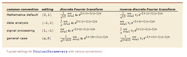
I concluded in my preliminary data post that the ‘Convolve’ function has its limitations and will not work properly with complicated functions. That may be so with relatively obscure functions, but I was wrong in my example. When I computed the convolution the long way by taking the Fourier transform of the product of Fourier transforms, I used the ‘FourierTransform’ function. I should have used the ‘InverseFourierTransform’ function instead. A Fourier transform of a Fourier transform is not necessarily the same as the inverse Fourier transform of a Fourier transform.
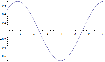
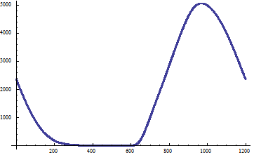
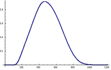
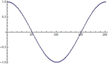
If f_1(x)=exp(-x)unitstep(x) \quad f_2(x)=cos(x), then through both methods I yield this plot:

Update

Mathematica file: https://vspace.vassar.edu/zerogoszinski/Update.nb

Vspace works better on Macs. If you are not using a Mac, please open the file from the Google Drive folder located at the end of this post. The file name is called ‘Update’.

Deconvolution:

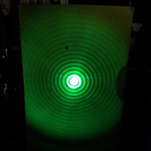
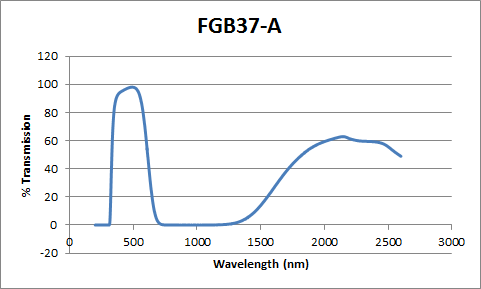
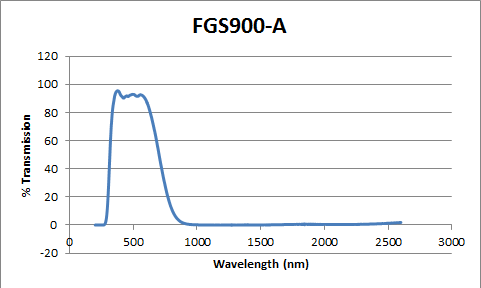
Convolution has applications in imaging, in that a blurry image is simply the convolution of the image and a lens or instrumental function. This function is also called ‘point-spread function’ (PSF). Convoluting two functions is simple since the individual functions are known. Deconvolution is the reverse process, in which you have a convolution and you want to extract the desired image. This requires an understanding of the blurring function, which requires understanding the system that is causing the distortion. Extracting the pure image is much more difficult since every blurring variable needs to be taken into account. A perfect PSF is impossible to determine, so accounting for this function requires good approximations (4). Deconvolution is very important in astronomy, since all data comes from optical based systems. Even a perfect lens convolutes images, as they have unique diffraction patterns. The best focused spot for a camera lens is called the Airy disk:

\theta=1.22f\lambda/d

f is the focal length, \lambda is the wavelength, and d is the diameter of the lens.

http://upload.wikimedia.org/wikipedia/commons/thumb/4/4b/Airy_disk_created_by_laser_beam_through_pinhole.jpg/480px-Airy_disk_created_by_laser_beam_through_pinhole.jpg

http://upload.wikimedia.org/wikipedia/commons/thumb/4/4b/Airy_disk_created_by_laser_beam_through_pinhole.jpg/480px-Airy_disk_created_by_laser_beam_through_pinhole.jpg


Here is an example of deconvolution in action:

http://opticalengineering.spiedigitallibrary.org/article.aspx?articleid=1183218

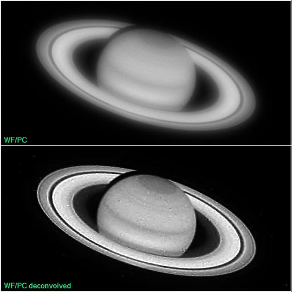
“Experience with the Hubble Space Telescope: 20 years of an archetype”
http://opticalengineering.spiedigitallibrary.org/article.aspx?articleid=1183218

A particularly cool example of the effects of PSF in astronomy is the black-drop effect during the transit of Venus. The black-drop effect is an optical effect where the planet seems to stick to the edges of the star during ingress and pull apart like taffy as it enters the surface. Calculating the transit time would determine the orbital period of Venus. Kepler’s third law would then determine the radius of orbit. Astronomers of the 18th and 19th century wanted to figure this out in order to determine the actual size of the solar system. The black drop effect made it difficult to determine the exact moment Venus entered the Sun’s surface. The cause for this effect was discovered to be mostly due to PSF (Schneider, G., Pasachoff, J. M., Golub, L., 2004, Icarus, 168, 249). Poor optics creates this optical illusion, and accounting for point-spread function [and solar limb darkening] eliminates this effect.


Created by Zeeve Rogoszinski using data taken from Big Bear Solar Observatory.  http://imgur.com/p19moKI

Click to see the animation.
Created by Zeeve Rogoszinski using data taken from Big Bear Solar Observatory.
http://imgur.com/p19moKI

As you can see convolution and deconvolution have important applications in optics. Light beams get distorted as they pass through matter, and the scientist needs to be able to determine what exactly he or she is looking at. If I had the time I would have tried to deconvolute my convolution in the previous post, and try to extract one of the optical filters. I would have first assumed I knew what the second filter looked like, and try to work out the procedure from there. I would then assume I have no idea how the filters behave, and try to blindly deconvolute the filters. This would require looking into the theory behind deconvolution in a more rigorous manner.

Transit Paper:

http://web.williams.edu/Astronomy/eclipse/transits/Schneider_jmp_lg_Icarus2004.pdf

All of my data:

https://drive.google.com/folderview?id=0BxRRP3LUVuftVmFCcnNPMWFhU1k&usp=sharing
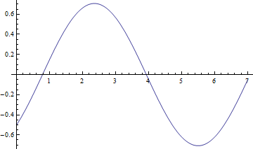
Share

Final Results: Convolving Optical Filters

Optical Filters

Now that we have the theory down, let’s apply convolution to actual data. The model here is two optical filters placed on top of each other. The light beam will go through both filters, and come out the other side somewhat convoluted. I have chosen two optical filters from thorlabs:

  • Item #FGB37-A: BG40 Colored Glass Filter, AR-Coated: 350 – 700 nm
  • Item#FGS900-A: KG3 Colored Glass Filter, AR-Coated: 350 – 700 nm

The plots of their transmission percentage as a function of wavelength are shown below:

FGB37A FGS900A

Notice the first plot down does not tend to zero as the wavelength increases. My hypothetical light beam will have a wavelength of around 500 nm, so I cropped out the two peaks from each plot from 200 nm to 1000 nm. I also added 200 zeroes to each end extending my plots from 0 to 1200 nm. I did this so that the transformations would have as little noise as possible.

Convoluting the two functions requires using the exact same method described earlier, but instead using discrete Fourier transformation. My first attempt at convoluting these two plots failed. The convolution gave me complex solutions, and I need my solutions to be real. I tested the method on two Gaussian functions by extracting artificial data points through the function ‘Table’. The list of data presented was not in the same format as the imported optical filter data. Mathematica does not like Excel, and the data imported was in the format of a list of 1×1 matrices of each point [The data also needed to be one dimensional, so the x-axis represents data point number. Fortunately the amount of data points is equivalent to the range of wavelengths, so for all intents and purposes the x-axis represents wavelength]. To bypass this confusion I saved my data as a text file and imported the list as a list. For example:

a = Import[“C:\\Users\\Zeeve\\Desktop\\EM Project\\FGB37-A test.txt”, “List”]

The data is now real. It should also be noted that the default setting for the Fourier transform is not the convention for data analysis. This requires using the tool FourierParameter to change the range from {0,1} to {-1,1}.

Capture


This is what my data looks like:

first attempt


The y-axis is the transmission percentage, and the x-axis is the wavelength.

Notice the peak is around 1000 nm. It turns out that the inverse discrete Fourier transform of the product of two Fourier transforms of data is not the convolution of the data. It is actually the cyclic convolution of the two data sets. If you go back to the original definition, one of the functions in the integral of the convolution is shifted by some value x’.

f_{1}(x)\ast f_{2}(x)=\int_{-\infty }^{\infty }\!f_{1}(x')f_{2}(x-x')\mathrm{d}x'

Notice also the y-axis and how it extends to beyond 5000. This is because my normalization constant was wrong. The square root of 2 Pi in the convolution algorithm is a normalization constant for Gaussian functions. Correcting this was simple. I used the ‘Normalize’ function to normalize my Fourier transforms, and used the product of those results:

v = Normalize[m]*Normalize[n] instead of c=Sqrt[2 Pi] m*n

Correcting the former issue is trickier. I need to cycle the function back to peak at around the 500 mark. I admit I am not familiar with the mathematically correct method of correcting this error, so I ball-parked it. The peak needs to be around 500 nm since the original data peaked at around 500 nm. Cycling the curve backwards required outside help. I used the method described in the first answer here: http://mathematica.stackexchange.com/questions/33574/whats-the-correct-way-to-shift-zero-frequency-to-the-center-of-a-fourier-transf .

The method uses the function ‘RotateRight’ to cycle a range of data a certain amount of points. My range of points extends from 0 to 1200, and I cycled 400 points. Now I have a plot where the x-axis is pretty much the correct wavelength for its corresponding value (although the values are off by a factor of 100, which is fine since it is simply a normalization correction), which is the convolution of the two optical filters:

convolution optical


Again here the y-axis is the transmission percentage, and the x-axis is the wavelength. The y-axis is off by a scaling factor.

For a complete transcript of the convolution, please check out the Mathematica script:

https://vspace.vassar.edu/zerogoszinski/Optical%20Filters.nb

Here are the text files:

https://vspace.vassar.edu/zerogoszinski/FGS900-A%20test.txt

https://vspace.vassar.edu/zerogoszinski/FGB37-A%20test.txt

Future:

For my conclusion I will discuss about deconvolution and some expansions on convolution.

Note: If the files do not work for you, I have uploaded all of my files to Google Drive which can be accessed in the conclusion. The concerning files are the Mathematica script ‘Optical Filters’, and the two text files ‘FGS900-A test’ and ‘FGB37-A test’. 


Share

Preliminary Results: Convolution and the Limitation of Mathematica

Update: See Conclusion

My preliminary results demonstrate the convolution of two arbitrary functions. There are two ways of convoluting functions in Mathematica. The first method is through a tool called ‘Convolve’, and the second method is through the product of two Fourier transforms as discussed in the previous post.

Example 1:

In this example I will demonstrate the convolution of two Gaussian functions of arbitrary widths:

y_1(t)=exp(-9t^2) \qquad y_2(t)=exp(-t^2)

The first method is simple. Plug in the two equations into the command ‘Convolve’ along with the necessary parameters. When I did this I got the function:

f(w)=\sqrt{\frac{\pi}{10}}\cdot exp(\frac{-9w^2}{10})

The second method requires finding the product of the Fourier transforms of the functions, then taking the Fourier transform of the product. The Fourier transforms of the two functions are as follows:

f_1(w)=\frac{1}{3\sqrt{2}}\cdot exp(\frac{-m^2}{36}) \qquad f_2(w)=\frac{1}{\sqrt{2}}\cdot exp(\frac{-m^2}{4})

Taking the Fourier transform of the product of these two functions and \sqrt{2\pi}, yields:

f(w)=\sqrt{\frac{\pi}{10}}\cdot exp(\frac{-9w^2}{10})

Both methods yield the same result, which is what should happen every time.

Example 2:

In theory any convolution of two functions adheres to the relationship:

{\widehat_{f_{1}\ast f_{2}}} (x)= \sqrt{2\pi}\;{\Phi_1}(k)\cdot {\Phi_2}(k)

Using paper and pencil and a lot of free time will demonstrate that this relationship is true. In practice, using a computer program to do the work for you could lead to some issues. Mathematica is limited by the sophistication of its algorithms, and convoluting simple functions can only take you so far. In this example I will demonstrate the limitations of Mathematica. Here I will be using the following functions:

f_1(x)=exp(-x)unitstep(x) \qquad f_2(x)=sin(x)

The unitstep function is the Heavyside step function which constrains the exponential function to the first quadrant. Convoluting the two yields the following function:

\frac{1}{2} (-cos(y)+sin(y))

EX2 1

The second method gave a slightly different result. Taking the Fourier transform of each function, multiplying them together, and then taking the Fourier transform of that function yielded:

\frac{1}{2} (-cos(y)-sin(y))

EX2 2


Both methods worked in the previous example, but here there is a sign change. I tried many different combinations of functions, and most of the time the two convolutions did not match. In fact, most of the time the first method did not give a clear result at all. Sometimes it did not compute the convolution, and sometimes the answer was obviously ridiculous. Fortunately, the latter method always gave an answer. To check to see if the latter method is reliable I redid the calculation using actual data points. I could not do the former method in a similar fashion because no such appropriate tool exists.

I used the ‘Table’ tool to give me a set of values from the two functions above. Here are the plots of the two data sets :

EX2 3      EX2 4


Taking the Fourier transform of each function yields complex values, and so I cannot graph those. The plots of the square of the Fourier transforms are not interesting. After going through with the latter method I came up with this plot:

EX2 5


This result is the same as in the previous attempt through analyzing functions. Considering Mathematica is well suited to handle data, and has a large library of Fourier analysis tools, I am confident that this method will provide the proper results for my future work.

Future

My next attempt will be to demonstrate the convolution of two optical filters. Thorlabs provides raw data of the transmission percentage as a function of wavelength for each filter. I will use the latter method to convolute the two filters, an then discuss how one would try to attempt to deconvolute the convolution.

Mathematica Script 

https://vspace.vassar.edu/zerogoszinski/Preliminary.nb

Share

Project Plan: A Guide To Convolution In Action

Description of project

Convolution is the theory behind interpreting the data presented. When physicists use optical tools for their experiments they need to understand whether the optics they are using will transmit the proper information. In practice one is limited to the material of the filters, as the wave fronts get distorted by the material they pass through. In order to be able to work with what you have, physicists model their possible optics layout before purchasing the optics. To retrieve the desired information physicists model the convoluted wave front, and then prepare a good deconvolution mechanism that in practice should yield the necessary data. This project is an attempt to understand convolution and deconvolution of electromagnetic waves through optical filters. I will be exploring the theory behind convolution, demonstrate examples of convolution, attempt deconvolution of a convoluted distributions, and then hopefully show a real world example of actual optical filters.

Theory

Convolution is the mixture of functions that individually have known Fourier transforms. A Fourier transform is the transformation of a square-integrable function f(x) 
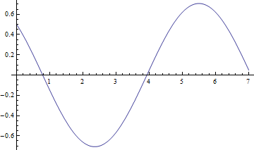
from one domain to another (5). It is defined as such:

f(x)=\frac{1}{\sqrt{2\pi}}\int_{-\infty }^{\infty }\!\Phi(k)e^{ikx}dk \qquad \Phi(k)=\frac{1}{\sqrt{2\pi}}\int_{-\infty }^{\infty }\!f(x)e^{-ikx}dx

Both the function and the Fourier transform describe the same system though under different but related spaces (See: Plancherel’s Theorem). The advantage is if you have a machine that measures time but you are trying the measure the system as a function of frequency, then you can measure the system with that machine and simply take the Fourier transform of your data. Unfortunately, the deviations of the Fourier pairs are bounded by the uncertainty principle. A function with a narrow spread will yield a transformation with a wider spread, and vice versa.

\sigma^2_\Psi\sigma^2_\Omega\geq\left(\frac{1}{2i}\langle[\hat{\Psi},\hat{\Omega}]\rangle\right)^2

where \hat{\Psi} and \hat{\Omega} are two arbitrary operators, and \sigma_{i} is the standard deviation.

The definition of a convolution of two functions is defined as follows:

f_{1}(x)\ast f_{2}(x)=\int_{-\infty }^{\infty }\!f_{1}(x')f_{2}(x-x')\mathrm{d}x' \\ \\ \Phi_{1}(k)\ast \Phi_{2}(k)=\int_{-\infty }^{\infty }\!\Phi_{1}(k')\Phi_{2}(k-k')\mathrm{d}k'

The convolution theorem then states that the Fourier transform of a convolution is the product of the Fourier transforms to a factor of \sqrt{2\pi}. Similarly, the Fourier transform of a product of functions is the convolution of the Fourier transforms (5):

{\widehat_{f_{1}\ast f_{2}}} (x)= \sqrt{2\pi}\;{\Phi_1}(k)\cdot {\Phi_2}(k)  \qquad {\widehat_{f_{1}\cdot f_{2}}} (x)= \frac{1}{\sqrt{2\pi}}\;{\Phi_1}(k)\ast {\Phi_2}(k)

The implication of this theorem is if any arbitrary curve can be expressed as a product of functions with given Fourier counterparts, then it can undergo deconvolution to yield the desired data as represented by known functions (3).

f_{1}(x)\ast f_{2}(x)\rightleftharpoons \Phi_{1}(k)\cdot \Phi_{2}(k)

Timeline

 All work will either be done on my computer or at the sci-vis lab.

Week 1: I will become familiar with Professor Magnes’s MATLAB script and reconstruct it in Mathematica. I will use the information provided for me in the texts to create new examples of various convoluted distributions. I will also provide an introduction to the theory that pertains to my project.

Week 2: By now I should be familiar enough with Mathematica to display some cool examples. I will attempt to provide an example of real world convolution of two optical filters from thorlabs. In practice convolution of two actual filters is not as easy as adding two equations. I will need to figure out how to generally apply my ideal examples to sets of data.

Week 3: I will now attempt to demonstrate the deconvolution of a distribution. I will show this by using one of my previous examples. In theory I should be able to demonstrate proper deconvolution of two functions.

Week 4: Now that I have demonstrated deconvolution, I should be able to demonstrate deconvolution of the data I had previously showed in convolution form. This would be very tricky but hopefully I should be able to succeed.

Week 5: I may be setting the bar up too high, so possibly some of my work will take more time than expected. I should be finished with everything now. Here I will tweak my project, and conclude my demonstration.

Note: I may stray from my timeline, but that is only because I got caught up in an interesting phenomenon. Should I decide to alter my direction, I will update my timeline accordingly.

Resources

Will be updated if necessary

(1) Griffiths, David J. Introduction to Electrodynamics. Upper Saddle River, NJ: Prentics Hall, 1999. Print.

(2) Hecht, Eugene. Optik. München: Oldenbourg, 2001. Print.

(3) James, J. F. A Student’s Guide to Fourier Transforms: With Applications in Physics and Engineering. Cambridge: Cambridge UP, 2011. Print.

(4) Pedrotti, Frank L., Leno S. Pedrotti, and Leno Matthew. Pedrotti. Introduction to Optics. Upper Saddle River, NJ: Pearson Prentice Hall, 2007. Print.

(5) Sadun, Lorenzo Adlai. Applied Linear Algebra: The Decoupling Principle. Providence, RI: American Mathematical Society, 2008. Print.

Question to the reader: Is the verb of deconvolution: deconvolve or deconvolute?

Share

Project Proposal: Modeling Optical Filters

When analyzing the brightness of a star, or a mode of a laser beam we observe the effects of that object. In this case we gather photons, and we use tools to gather as much radiation as possible. This data is then transmitted onto a screen to see a representation of what is actually going on. When an electric signal is sent to an oscilloscope, are we actually seeing the signal? A spectrum of light must enter through a series of optical and electrical things before being displayed, and those things can and do distort the image. These are optical filters. Sometimes this is done intentionally to block out certain frequencies, but other times the distortion is unavoidable. By understanding the convolution of electromagnetic waves one can isolate the desired data from the signal presented. I will model using Mathematica different spectra and examine how convolution and deconvolution work as means of setting up usable data.

Share