MONTE CARLO METHODS FOR ELECTRON TRANSPORT
PHYS 375
WANJIRU GACHUHI (SHISHI)
With the growing technology, semiconductor devices are becoming smaller and are being operated on higher electric fields. These high fields result in high-speed carriers which are more difficult to analyze analytically. Computational methods such as the Monte Carlo Method for electron transport have, therefore, become necessary to understand the Physics of carriers within semiconductor materials.
In solids, the probability of finding a carrier, in this case, an electron located at position r, at time t, with a momentum p is given by f(r, p, t) [1]. f(r, p, t) is the probability function and is derived by solving the Boltzmann Transport Equation (BTE). The BTE [Eq 1] gives us the position, energy and momentum of carriers under the influence of electric fields and as a result of collisions. The distribution function depends on various factors such as the location, energy, direction, and energy band of electrons in a semiconductor. These numerous factors, together with the collision term on the right in Eq 1, make the BTE impractical to solve analytically. These factors also make it impossible to solve using numerical discretization techniques. Eq 1 can, however, be solved numerically using the Monte Carlo (MC) Method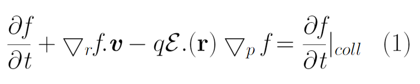
Monte Carlo Method is a computational method that makes use of random sampling to simulate numerical solutions. This differs from other computational methods such as the Euler, Euler Cromer, and Runge Kutta that make use of numerical discretization. The Monte Carlo (MC) method has been shown to give an accurate solution to the BTE [Eq 1], provided that a large number of particles are simulated [1]. The MC method for electron transport involves four stochastic processes each generating random numbers that mimic the underlying Physics of electron transport in a semiconductor. These stochastic processes are: generating free flight times, selecting the type of scattering that occurs, and randomizing the orientation of scattered electrons. This project focuses on the Physics and the computational methods that give the position, energy, and momentum of electrons under the influence of an electric field and scattering events in a semiconductor.
When an electric field is applied to a semiconductor, an electrostatic force is generated thereby causing the electrons to accelerate in the semiconductor [Eq 2]. The position, energy, and momentum of the electrons are initially influenced by the electric field only. These electrons move within the semiconductor until a collision occurs (scattering event) resulting in a change in position, energy, and momentum of the electrons. These scattering events can be caused by various factors, such as impurities, or the emission/absorption of phonons. Identification of the type of scattering that takes place is necessary to determine the energy of the electrons after scattering. Once the type of scattering is identified, the position, energy, and momentum are updated. This post explains how the Monte Carlo Method was used to solve the BTE, thereby extracting the same information about the electrons as would have been obtained from the probability distribution function, f(r, p, t).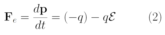
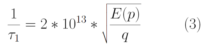
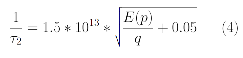
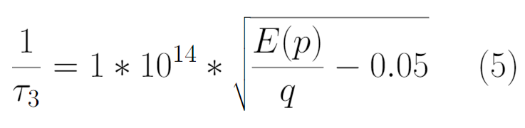
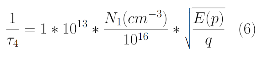
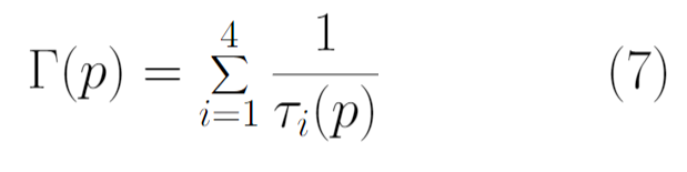
In a semiconductor, the free flight times of electrons must be the same as the time until their next collisions. An electron that has a free flight time of 3e14 s suffered a collision after 3e14s. The scattering rate is, therefore, necessary to accurately simulate free flight times of the electrons. Scattering can be caused by impurities in the semiconductor, or by phonon absorption or emission. In this case, we consider four real types of electron scattering. Acoustic Deformation Potential Scattering (ADP) in the elastic limit [Eq 3], intervalley scattering by phonon absorption [Eq 4], phonon emission [Eq 5], and Impurity scattering [Eq 6]. These are considered real scattering rates as they change the momentum of the electrons after scattering [1]. The total scattering rate of carriers is the sum of these scattering rates and is given by Eq 7 below. The total scattering rate is a function of the kinetic energy of the electrons as shown in Figure 1 below. We observe that particles with higher kinetic energies have higher scattering rates.

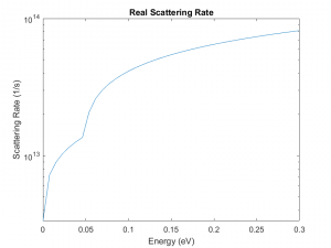
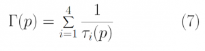 Figure 1: Real Scattering Rate vs Kinetic Energy

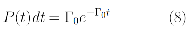
The probability that an electron does not collide within a given time-step is given by Eq 8 [1]. This can be solved computationally by choosing a random number (R1) that ensures that the probability of choosing the random number equals the probability of selecting a scattering event [1]. Assuming a constant scattering rate, Eq 9 gives the scattering times that are generated from random numbers ensuring that the distribution of the scattering times (t) will be equal to the distribution of P(t).
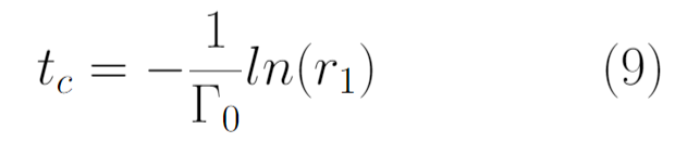
This was performed in Matlab by generating 10,000 random numbers between (0,1) corresponding to 10,000 electrons. The constant scattering rate (Γ0) was assumed to be 3e14. Eq 9 was used to generate the free flight times. A histogram of the free flight durations was plotted as shown in Figure 2. This distribution was equal to the distribution of P(t) [Eq 8], which ensured that the flight times that were generated correspond to the scattering rates of the electrons. The average flight time for flight times in Figure 2 is 3.32e-15 which was approximately equal to 1/ Γ0.
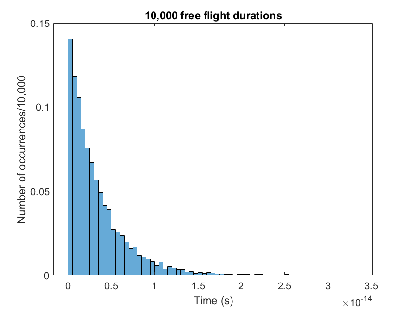
Figure 2: Histogram of free flight times of 10,000 electrons
Once the random flight times were generated, a Matlab Code was written to simulate the position, momentum, and energy of 10,000 electrons under the influence of a constant electric field of -1e-12V/m in the -z-direction. This resulted in a change in position and momentum in the +z direction. Eq [10],[11],[12] were used to update the momentum, energy and position of the electrons under the influence of the electric field. Figure 3 below shows the change in position and momentum of 20 electrons in the z-direction.


Figure 3: Momentum vs time for 20 electrons with an initial kinetic energy of 0.15eV
Although assuming a constant scattering rate ensured that we could use Eq 9 to find the free flight durations, that did not capture the real scattering rate. The real scattering rate changed as a function of time as seen in Figure 1. A fictitious scattering rate was added to the real scattering rate to ensure that the scattering rate Γ0 remained constant [1]. This is known as the Self Scattering Technique Eq 13. The fictitious, self-scattering rate does not alter the position or momentum of the electrons and was only added to the real scattering rate to allow us to use Eq 9 to find the free flight times [1]. ![]()
At the end of the free flight, scattering took place. Identification of the type of scattering that took place was necessary to determine the change in kinetic energy of the electrons. Both ADP and impurity scattering are elastic scattering processes, therefore the energy of the electron before and after collision is equal. However, intervalley scattering by phonon absorption and emission involves either absorbing or emitting a phonon after collision. Determining the type of scattering was also necessary to accurately simulate the position, momentum, and kinetic energy of the electrons after collision.
This was performed in Matlab by generating 10,000 random numbers between (0,1). A code was written to walk through the random numbers (R2), identifying the scattering type according to Eq 14 below. Eq 14 gives the conditions by which the different scattering types were identified. These conditions relate to the scattering rates obtained from Eq 3- Eq 7. A graph of the scattering types was obtained as seen in Figure 4. Among the real scattering types, intervalley scattering by phonon absorption was the most common type of scattering. This is consistent with other studies [1]. This step in the Monte Carlo Method assigned each of the 10,000 previously generated electrons a specific scattering mechanism that was necessary to determine the change in energy after collision.
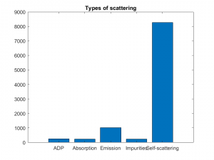
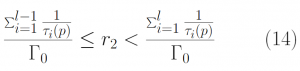
Figure 4: Types of Scattering in a semiconductor

Once the type of scattering was identified, the momentum was updated according to Eq 15. For inelastic collision, the change in energy was either due to absorption or emission of a phonon with an ∆E of 0.05 eV. The orientation of the momentum after scattering was also determined.
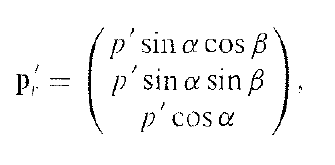
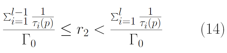
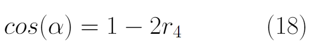
The orientation of the momentum was first determined on a rotated coordinate system where the z-axis was directed along the initial momentum. Once the new magnitude and orientation on this rotated axis were found, p was determined on the original coordinate system by using Eq 16. The orientation after scattering was found by generating two other random numbers, R3 and R4. R3 randomized the azimuthal angle according to Eq 17, and R4 randomized the polar angle according to Eq 18. The distributions of β and α were plotted as seen in Figure 5. β was uniformly distributed between 0 and 2pi while cos (α) was uniformly distributed between +1 and -1.

Figure 5: Distribution of azimuthal and polar angles for scattered electron momenta

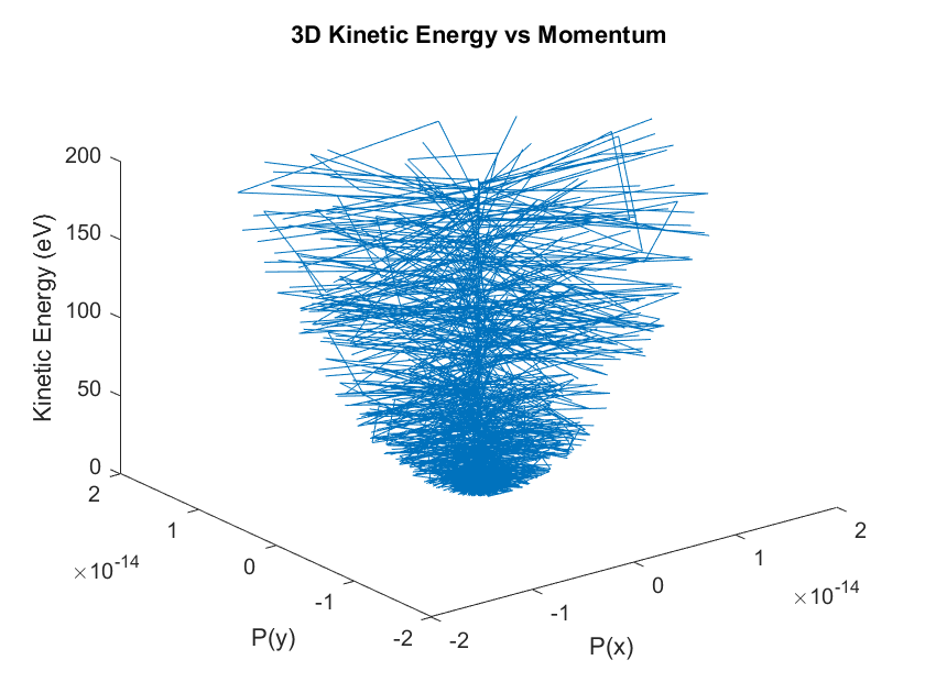
The updated magnitude and orientation of the momenta in all three axes were then determined using Eq 15 &16. A plot of the energy as a function of the updated momenta in the x and y axes was plotted as seen in Figure 6. A parabolic shape was observed which aligns with the assumption made earlier of parabolic energy bands. The average kinetic energy of the electrons in Figure 6 was 39.9693 eV while the average kinetic energy before collision was 39.9732 eV. A large change in the average kinetic energy was not observed because most of the collisions were a result of self-scattering which did not result in a change in momentum or energy after collision. The small difference of 0.0039 eV was due to phonon emission and absorption. In addition, the phonon energy of 0.05 eV was much lower than the kinetic energy of the electrons before collision (39.9732 eV) resulting in a small change in the total kinetic energy.

Figure 6: Kinetic Energy vs Momentum
In conclusion, the Monte Carlo Method was successfully used to simulate electron transport in a semiconductor under the influence of a constant electric field and scattering events thereby solving the Boltzmann Transport Equation. The position, energy, and momenta were obtained for electrons before and after scattering. Parabolic energy bands were also observed which was consistent with the assumptions made. This technique can also be useful when determining the type of energy bands. This is known as the Full Band Monte Carlo Method.
One limitation in this project was that the phonon energy and the electric field were chosen arbitrarily. Future work can investigate the effect of the energy, momentum, and position of electrons with a non-constant electric field. Similarly, calculations can be made to determine the energy of the phonons that are absorbed or emitted.
References
[1]. Lundstrom, M. (2010). Fundamentals of Carrier Transport. 2nd ed. Cambridge: Cambridge University Press, pp.247-279.