Author Archives: juvasquez

Audio Signal Processing – Conclusion

Goal:

Our final program takes an acoustic wave signal, strips out all audible frequencies using a Fourier transform, then shifts a range of the ultrasound frequencies into the audible range in order to qualitatively investigate the properties of the audio signal. Our initial goal was to record our own ultrasound frequency signals for analysis, but we were not able to procure a microphone sensitive enough to record ultrasound. Instead we choose an online video claiming to repel rodents by emitting an audio wave with ultrasound frequencies that effect rats (found here: https://www.youtube.com/watch?v=l5x1Bb9UTT0). On first inspection, the signal seemed to only play what resembled white noise, but we needed an accurate representation of the frequencies present in the audio file before making any more assessments. We hypothesized that the video did not contain ultrasound frequencies capable of repelling rodents.

Investigation:

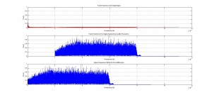
Using the frequency analysis methods we implemented earlier in our project we found that the video actually contained frequencies above 20 kHz. But we were still skeptical because these higher frequencies were about 80% less powerful than the frequencies present in the audible range. This may have been a tactic used to trick the user in believing that high frequency sounds were playing. We wanted to examine what the high frequencies sounded like so we took a 5 second clip from the audio file to scrutinize.

(Please find the 5 second clip here: https://drive.google.com/file/d/0B4quZV7NVNf7YU16blYwcUxXYXc/view?usp=sharing)

We started by removing any audible frequencies from the clip then shifted the ultrasound range into the audible. The resulting sound was again white noise, but at a lower volume.

(No audible frequencies: https://drive.google.com/file/d/0B4quZV7NVNf7clBFTlJIT1I5bzQ/view?usp=sharing , Shifted signal: https://drive.google.com/file/d/0B4quZV7NVNf7amhqVkZ6NjBtUXc/view?usp=sharing)

A qualitative analysis of this new wave does not lead us to believe this video would repel anything. White noise is not an abrasive sound unless played at extremely high volumes, but anything played at a high enough volume can be found abrasive. White noise is generally considered to be the exact opposite and there are white noise generators that are sold on the premise that they are calming and relaxing, and are used to help people focus or sleep. The video we analyzed is not exactly what we would expect in a rat repellent, it seems like this video aims to be more of an aid that would assist in rat mediation.

(code here: https://drive.google.com/file/d/0B4quZV7NVNf7cldUbG5WQUFWTXM/view?usp=sharing)
Virgin Wave

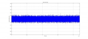
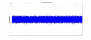
Here is the clip from the original 5 minute video. Notice the amplitude of this signal.

Analysis of Frequencies

Here are the various operations we performed on the Fourier transform of the clip.

Audio Signal Without Audible Frequencies

No audible frequencies are present in this new signal. Please note the difference in amplitude in this signal from the original signal.

Shifted Signal

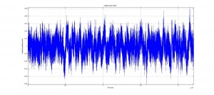
The new, shifted audio signal.

We then decided to make a code to demonstrate what a real rodent repellent signal might sounds like. We start by assuming that sounds that are irritating to humans are also irritating to rodents. A sound that is often considered to be annoying to us is a pair of high frequency sinusoidal waves that are similar in frequency but not identical. This is a very dissonant sound, and even at low volumes can grab the negative attention of someone around you (which can happen if you accidentally sound them in a public space while coding a rat repellent). So we also built a code that generates what we consider to be an abrasive sound, but is well above the audible range so we cannot hear it. We decided on the frequencies of a distressed rat baby (http://www.ratbehavior.org/rathearing.htm). Unfortunately, Matlab’s audiowrite function was not able to save this as a .mp3 file, so please download the code play and use the sound command found to play it on your machine.

(code here: https://drive.google.com/file/d/0B4quZV7NVNf7OW1kQld5QW1KVkk/view?usp=sharing)

 Future Work:

If we were to continue to research methods and applications frequency shifting we would write a code that transposes frequencies. Transposition maintains the harmonic ratios of the frequencies present in the wavefunction by multiplying them by a constant instead of linearly shifting them. Changing the sampling frequency at playback also maintain these ratios but in doing so, distorts the audio signal by stretching or compressing the wavefunction. Out next code would have been to transpose frequencies without changing the length of audio sample. We would also like to to detect our own ultrasound frequencies with an ultrasound microphone for qualitative analysis.

Share

More Results – Shifting Frequencies Up and the Effects of Linear Shifting

Last week we used Matlab to record original audio file using a desktop computer microphone.

Please find the code here:

https://drive.google.com/a/vassar.edu/file/d/0B4quZV7NVNf7MFFWU0lMVGpEZ00/view?usp=sharing

Upon contacting the appropriate members of the Vassar physics faculty, it has come to our attention that the school does not posses an ultrasound detector. We then tried extremely high sampling rate using a normal microphone to try and capture ultrasound frequencies with no avail.

instead we took a signal with a frequencies in the infrasound range, even though it was not originally a sound vibration. specifically we took the power signal from a red and green laser inside an interferometer from the Fourier transform spectroscopy lab and turned it into a wav file. We then took the fft of that wave, and used the circshift function on the fft data to moved it up in the frequency spectrum to the audible range.

Please find the code and necessary audio file here:

https://drive.google.com/open?id=0B4quZV7NVNf7LXJqNERTZEpYckU&authuser=0

https://drive.google.com/open?id=0B4quZV7NVNf7VW5LTVczUUNablVBMzkzdmJWOWctclRxSGdZ&authuser=0

Shifting Frequency Linearly

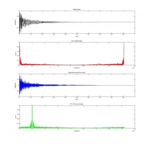
Notice the shape of the shifted signal. We hope to account for the error in the audible signal by accounting for the harmonic ratios.


This method of frequency shifting does not change the amount of time the file takes up, but it does not maintain the ratio between the frequencies. Because the shift is linear, it changes the harmonic interval between the frequencies. An example of this would be an interval of an octave. if you have a frequency of 200 Hz the next octave of the same musical pitch would be twice the frequency 400 Hz. If you shift both of those frequencies up linearly by 100 Hz you would have frequencies of 300 Hz and 500 Hz. The ratio between the two new frequencies is different than in the original. The effect is made noticeable in the following examples:

Shifting up 34 Hz

Shifting Up 39 Hz

Shifting Up 44 Hz


The next step is to maintain the harmonies using a by keeping the ratios constant as we shift the frequencies. Matlab’s findpeaks function will aid us in performing this task.

We decided to make a signal of our own and play with changing frequencies to see how it effects the wave and its Fourier transform.

Please find the code here:

https://drive.google.com/open?id=0B4quZV7NVNf7SEZqeEtTY2dRU2s&authuser=0

Share

Audio Signal Processing – Preliminary Data

We have used Matlab to read, write, plot, and play audio files. We begin by taking the fast fourier transforms (fft) of these audio files and manipulated the locations of the frequencies using different methods.

Original Sample


1. changing the sample rate

Audio files have a given sample rate at which they are recorded, usually 44.1 kHz. If you play the audio file back at a different sample rate the pitch of the audio is changed. For example, if you play the audio at 88.2kHz the frequency of the sound is higher due to the wave function being read faster; this however also changes the length of time of the audio sample (something we want to avoid in our project).

 Half the Sample Frequency

Twice the Sample Frequency


2. upsampling/downsampling

By adding samples to the array of the sound file, but playing it back at the original sampling rate, changes the pitch of the audio file when played back. This is done by either adding elements to the array every nth element (upsampling) or deleting every nth sample of the array (downsampling). Upsampling decreases the frequency and downsampling raises the frequency. This also changes the amount of time the sound file takes on playback because it changes the length of the array being read, but not the speed at which it is read.

 Upsampling

Downsampling


3. phase shifting

When taking the fft of a wavefunction, you get an array of amplitudes, and the matrix element it the frequency of which the amplitude value is representative. When phase shifting , the elements get shifted down or up and the elements at the end of the array are looped to the beginning.

Made in Matlab

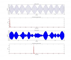
The top two graphs show the original signal and its Fourier transform. The bottom two graphs illustrate the effect of phase shifting.

 Phase Shifting


4. finding peaks

If you use a peak finding function of the fft of a wavefunction, you could use those values to rebuild the signal using sinusoidal function of frequencies of the locations of the peaks. if you were to shift the values of those peaks before rebuilding the wavefunction, you could in theory create a wavefunction of a different pitch without changing the amount of time. We have yet to implement this method, but it is part of our next trials.


Please find the Matlab code here:

https://drive.google.com/a/vassar.edu/file/d/0B4quZV7NVNf7ako4RlBkeUNETXc/view?usp=sharing

Sound File Source:

http://eleceng.dit.ie/dorran/matlab/

Share

Ultrasonic Analysis

Introduction

The Fourier Transform (FT) is a mathematical tool that takes a signal in a time domain and decomposes it into it’s frequency domain. Below is the definition of the continuous FT of $x(t)$ to $X(f)$,

$X(f) = \int_{-\infty}^{\infty} x(t)e^{-i2\pi ft}~dt$.

This comes in handy when trying to analyze signals found found in electrical circuits, diffraction patterns, and sound waves. We intend to use the same techniques to study and manipulate sound signals found in the ultrasound domain.

Acoustics is the study of the generation, transmission, and reception of vibrational waves in a medium. Mostly acoustics is associated with sounds we can hear, but vibrational waves can occur outside of the range of human hearing. Humans detect vibrational waves from a range of 20Hz to 20,000Hz as sound waves, but any vibrations occurring above or below this frequency band go undetected by our ears. Ultrasound is any sound vibration above 20,000 Hz, it shares all physical properties of audible waves other than human perception.

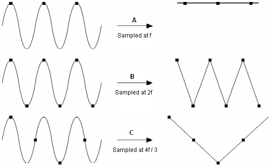
The standard sampling rate used by computers to capture sounds vibrations is 44.1 samples per second. It is necessary to capture signals slightly above the nyquist frequency. The nyquist limit is a result of having to sample a wave at least twice per cycle to represent the wave without aliasing. The nyquist limit will be an important part of accurately recording the waves because of the high frequency content of ultrasound.

Here is a small demonstration the shows the importance choosing a sampling frequency

Determining the sampling rate of these signals will be an important experimental consideration, but we know it will be much greater than 44.1 samples per second.

Goal

We will be processing a variety ultrasound frequencies and attempt to pitch shift them down (without loss of quality) to the audible range for listening.

Timeline

Week 1 (4/6 – 4/12)

Gather necessary resources and work on problems from the texts to gain requisite background information and foundational code to perform effective analysis of ultrasound signals.

Week 2 (4/13 – 4/19)

Continue to work on the code. Study sources that generate ultrasonic sound vibrations, and methods of recording them.

Week 3 (4/20 – 4/26)

Record ultrasound signals and convert recordings into a suitable file for matlab to take in for analysis. Attempt to analyze and pitch shift the signal and play it back. Debug errors.

Week 4 (4/27 – 5/3)

Continue analysis on a variety of signals recorded during week 2.

Week 5 (5/4 – 5/10)

Presentation and write-up.

Resources

Fundamentals of Acoustics 4th Edition by L. E. Kinsler and A. R. Frey

A Student’s Guide to Fourier Transforms 3rd Edition by J. F. James

Fundamentals of Digital Signal Processing Using MATLAB®, 2nd Edition by Schilling/Harris                  

Computational Physics 2nd Edition by Nicholas J. Girodano, Hisao Nakanishi

The Computer Music Tutorial by Curtis Rhodes

Share