Author Archives: elkim

Review of Sarah and Lily’s Project

I appreciate astronomy as much as any Vassar physics student, and I think that your original goals were pretty comprehensive and distinct. The kepler laws are a pretty well-documented and studied set of physics, and it seems a challenging and rewarding problem to solve them numerically, especially since a few Vassar classes (PHYS 210, Astro 230) focus on solving them analytically. The analytical solutions, if I am remembering correctly, were pretty taxing and so using a numerical approximation seems a good way to solve a pretty complex problem.

Project Plan:

It seems to me as though you guys had a pretty firm grasp on the kinds of concepts and equations that would be necessary to solve these problems. I do have a couple questions:

  1. Did you consider simulating the effects of tidal forces or at least just the magnitudes of tidal forces? Especially in the moon/earth/sun system, tidal forces seem to be a pretty central piece of physics. I think it would have been cool to see these forces in the original two-body program and then even cooler to note how the moon, with a relatively small mass (at least compared to the sun), so intensely affects the tidal forces on the Earth.
  2. I’m not sure why you chose to try to solve the three-body system before solving the system with the two large masses. Having written the original program, would it not have been trivial (or at least logical) to then just increase the mass of the Earth and give the sun some sort of initial velocity?

Preliminary Results:

The euler-chromer method seems to me to be a pretty effective way of solving these differential equations. I like the visuals that you’ve provided to display the results, especially the juxtaposition of the radius plot next to the more visually gratifying plot of the Earth’s actual motion. It is really cool to see this radius plot side by side, and an effective way to verify that your solution seems to be correct. Once again, a couple more questions:

  1. You note that you intentionally left out the masses of the sun and earth as the sun’s mass is so large in comparison. Similarly, you’ve also assumed that the sun does not move. These seem like pretty crucial assumptions, and I think it would have been good to show that your solution is still correct and that the sun is only moving a little bit when it is allowed to move. I say this also because as I noted before, the final goal for your project was to create a program that might have simulated two massive co-orbiting bodies. Wouldn’t you have had to write an expression for masses and an initial velocity anyway? Seems to me like this could have been a pretty key step in the grand scheme of your project.
  2. Did you consider a different method besides euler chromer? Since the euler chromer only evaluates derivatives at the beginning of an interval, could this have had some effect on the results you were getting?

Final Results:

I give you props for solving the system using an analytical method; it seems that you’ve shown a situation where the numerical approximation of the motion might actually be more complex. I think you also did a great job problem-solving and exploring possible sources of error, it seems like your search was really comprehensive and that you checked every piece of your code. One comment:

  1. Why did you choose to use the “straight-line” model when simulating just the Earth and the Moon? Does this really add anything to solving the problem? Isn’t the Earth and Moon system practically identical to the Earth and Sun system? Once again, I feel like this is where not using mass and initial velocity in the initial problem may have come back to hurt you. That seems to me like a pretty crucial step that could have affected the whole project,

Conclusion:

I like your discussion of the methods you used. This, to me is the most important part of physics, evaluating whether or not what you have done is useful or correct. Since the whole point of a numerical approximation is to lessen the taxing nature of the analytical solution, it is especially important to identify problems for which it is not effective. That being said, why did you abandon the third part of your project? Instead of spending so much time trying to fix the second part, might it not have been better to see if the Euler-Chromer method is effective when evaluating that kind of problem? Overall, really good job and good physics.

Share

Project Plan: Monte Carlo Method and its applications in Finance

Theoretical Motivation:

During the final stages of the Manhattan Project, Stanislaw Ulam and John Von Neumann developed the Monte Carlo method in order to calculate on average how long it would take for a neutron to collide with the nucleus of an atom when projected into a given substance. Named after the famous Monaco casino, Monte Carlo methods are often used to describe systems that have a set range of inputs and parameters, the specifics of which are unknown. The method inputs random or pseudo-random values into the system over and over again to see if a certain trend emerges when certain combinations of values are chosen. Often, Monte Carlo methods are used to simulate systems in physics that have many coupled degrees of freedom, such as radiation and fluid dynamics. However, many social scientists have since begun to use Monte Carlo simulations to predict the ways that certain trends develop, particularly in the world of finance and economics.

The Ising model emerged from the study of ferromagnetism, providing a way to study the interactions between adjacent atoms with discrete magnetic spin numbers. Since each spin influences its surrounding neighbors, these systems are modeled by creating a grid of cells that influence the cells around it based on a specific set of laws or equations. In the context of physics, the Ising model has since expanded from the field of ferromagnetism into thermodynamic phase transitions and other related fields. Like the Monte Carlo method, it has also been commandeered by the finance community to map the progress of interrelated variables and actors in an economic system. It does so by defining a set of actors governed by mutual economic and financial laws.

Finally, in the world of finance, volatility refers to the way that a financial instrument’s price changes over time. Many traditional models of volatility follow a deterministic approach in which the price of a financial security (any type of financial asset) has a constant volatility over time. However, these models often fail because the volatility of any given security is in reality stochastic over time and evolves due to the contributions of many factors, some of which cannot be seen directly. To account for this stochastic volatility when determining the price of financial assets, economists have often turned to Monte Carlo methods and the Ising model to predict the way interrelated, seemingly random factors evolve over time. Adam Warner and I plan to gain a preliminary understanding of the way that these methods transfer from physics to the world of finance.

Description:

I will begin my study by using MatLab to write very basic examples of both an Ising system and an independent Monte Carlo method, starting with the discussion in Giordano’s computational physics. I will then use a Monte Carlo simulation to solve a more rigorous physics problem, concerning the emission of radiation from an atom. This process is stochastic in nature, so I believe it will be a good precursor to looking at the kind of method necessary to solve a financial volatility problem. I will then attempt to model the volatility of a derivative security, a financial asset that depends on the prices of other more basic assets. Finally, if time allows, Adam and I will work together to develop an Ising model that describes an economic system.

Timeline:

Week 1 (4/6-4/12)

I will finish my research on the basic principles of the Ising Model, Monte Carlo Methods, and Volatility. I would like to have a comprehensive list of papers to reference and be ready to start working in MatLab.

Week 2 (4/13-4/19)

At this point, I will start to work on my models for the basic Monte Carlo and Ising problems. I do not think that these will be too rigorous and I hope to be able to display these in my first preliminary results report. I will need to figure out the kind of notation to use for this sort of computation.

Week 3 (4/20-4/26)

By then, I should be ready to start my model of atomic radiation. This will help me get a good grasp on how to approach a stochastic system in MatLab and should be an example of some pretty interesting physics concepts. I hope to get this into my preliminary results as well, but am less certain.

Week 4 (4/27-5/3)

Now, I will attack the meat of my project. I will use all of the concepts I have worked with up to this point to model the stochastic evolution of the volatility of derivative security.

Week 5 (5/4-5/10)

This week I should be able to finish the model described previously. If all goes according to plan, I will have time to work with Adam on characterizing how an Ising model would be able to describe the evolution of interconnected securities and the decisions made to give them prices.

Sources:
1. Computational Physics, Giordano and Nakanishi
2. Physics and Financial Economics (1776-2014): Puzzles, Ising and Agent-Based models
D. Sornette (ETH Zurich)
3. University of Virginia: Introduction to Atomic Simulations, Leonid Zhigilei
4. Probability Review and Overview of Monte Carlo, Martin Haugh
5. Monte Carlo Methods for Security Pricing, Phelim Boyle, Mark Boardie, Paul Glasserman
6. Monte Carlo simulation of the atomic master equation for spontaneous emission
R. Dum, P. Zoller, and H. Ritsch

Share

Project Proposal: Applying Physics to Problems in Financial Markets

Many economists work on problems where they cannot be sure how different factors affect each other. In the context of physics, the Ising model is used to study the interactions between bodies that make up complex systems. A number of internal and external factors influence the way these bodies interact with each other to affect the whole system. There are several ways to solve Ising models, but one of the most pragmatic is the Monte Carlo method, which calculates the probability of certain factors occurring over and over again at varying probabilities until the system reaches an optimal level.  Adam Warner and I would like study the ways these techniques aid problems done by economists. First, we will use MatLab to model a simple Ising system in the context of a physics problem relating either to magnetism or phase transition. From there, we will each look at different ways that Monte Carlo methods and Ising Models apply to financial models. This analysis will include a survey of utility-based decision making, market booms and crashes, and the volatility of stock pricing. We hope to compare the results we obtain through our MatLab programs to established studies done by financial institutions.

Share

Railgun Physics: Final Thoughts

Having completed this project I have several thoughts about what I did, what I could’ve done, and what I want to do in the future. This project taught me a lot about physics, a little about engineering, and a great deal about modeling and the work and mindset necessary to complete projects of this nature.


The physics I got to explore as part of this project was extraordinary. Before I began, I knew little about railguns, only that they used extremely powerful electromagnetic forces to create massive destruction. The first part of my results showed an interesting but unsurprising result. The initial current originating from the capacitor was extremely large; a capacitor charged to 1.8 coulombs generated an initial current of over a million amperes. At first, this value seemed a bit high, and in reality was most likely a little higher than we expected. However, within a matter of several hundredths of a micro-second, this value immediately dropped to several hundred thousand amperes and then even lower values shortly thereafter. The current dropped even further when the length of the rails changed or when the cross sectional area of the rail decreased. Doing both of these, something that is realistic over time, lowers the current even more drastically. Therefore, we saw that the rail gun really does involve an initial intense burst of current followed by no further circuit action. We then saw the effect of EMF. At the beginning of the project, I thought that EMF would be too hard to derive and almost discounted it. Having done it, I realize that this decision would have been poor, as EMF ended up playing a huge role. The EMF induced a current that reduced the original current by almost 3/7ths, a substantial amount. Once again, this factor was dependent on the length of the rails and conductivity of the material. Finally, the resulting magnetic field was extremely powerful but fell in line with all the other results we found. In the first moments of the circuit’s operation, an enormous magnetic field is generated, creating a large force for a very brief amount of time.  This occurrence made sense of course, as magnetic field depends on current. I am happy with these results, as they mirror the conceptual understanding of railguns I have developed during the course of this project; an enormous power lasts for an infinitesimal amount of time.

    Part of our project was not able to happen, of course. We had originally planned to build the small scale rail gun, but because of time and safety concerns were unable to. In the future when doing these kinds of projects I will be able to better adjust my plans for safety and for time. I also could have tried to make more 3D models of my models, but thought that the 2D representations made sense in the context of the project.

    In the future I would like to be able to derive equations of motion as functions of time. So many of the results I obtained were dependent on velocity and position. I adjusted for this by allowing these variables to be selected over a certain range; for example, using my model can tell you what the magnetic field of a railgun is at an exact time, position, and velocity. This result is very useful, but I would ideally like to be able to have position and velocity as functions of time as well. With more time and more math, specifically a greater knowledge of differential equations, I think I would be able to do so.

Share

Railgun Physics Final Results: A Dangerously Powerful Circuit

As my part of the project, I have successfully modeled how a railgun acts as a circuit. These results are interesting on their own, but throughout this post I will try to put them in context and show the various aspects of my results. In my preliminary data, I had derived the most general versions of the magnetic field of the rails, missing a good amount of necessary information. I modeled resistance, showing how it changes as the factors that compose it change. I will present the rest of my results by first introducing each necessary concept, and then showing how it is applied in one of two scenarios: a small-scale railgun and a military-scale railgun.

IMAG0129

Current from the Capacitor Setup:

As noted before, the original current in the circuit comes from a bank of capacitors of varying degrees of strength. The capacitor has an initial charge:

(1)   \begin{equation*} {Q_0} \end{equation*}

This charge will decrease over time, where

(2)   \begin{equation*} {Q=Q_0e^{\frac{-t}{\text{RC}}}} \end{equation*}

As we can see, the charge in the capacitor decays at an exponential rate proportional to the resistance of the circuit and capacitance of the bank. The higher these values, the longer it will take to discharge.

Now we can see that the current is time derivative of Q,

(3)   \begin{equation*} {\frac{\text{dQ}}{\text{dt}}} \end{equation*}

The result of this derivative is:

(4)   \begin{equation*} {o=\frac{Q_0}{\text{C$\rho $}\frac{(2L+2d)}{A}}e^{\frac{-t}{\rho \frac{(2L+2d)}{A}C}}} \end{equation*}

We will use this term “o” to refer to the current from the capacitor. We will model two specific scenarios, a small scale rail gun that we found online, and more massive versions of the rail gun that the military might use. Below is the model for current due to power supply of a small scale version with rails of .2m spaced .03m apart, and cross sectional area .0009m^2 with 10 450 microfared capacitors connected in parallel to store maximum charge.

Here you can see that the current from the capacitor is massive at first. It then drops very immediately over a very short period of time. The majority of the current is gone after a little over a nano second. As you can see, adjusting the length of the rails also causes the current to drop, meaning that as the projectile moves and the length of the rails in the circuit lengthen, the current drops tremendously. The same is true with the resistivity; rails made of aluminum draw a great deal more current than do the rails made from steel, the opposite end of the resistivity spectrum.

Now we will model the most prototypical version of the rail gun proposed and worked on by the navy. According to our research, the rails of this gun will be up to 10m long, spaced .8 meters apart, a cross sectional area of .01m^2, and be supplied by capacitors storing 33 megajoules of energy. Energy Stored in a capacitor is defined as:

(5)   \begin{equation*} {E= \frac{Q^2}{2C}} \end{equation*}

Which, knowing that 33 megajoules of energy is necessary, yields

(6)   \begin{equation*} {Q=8124\sqrt{C}} \end{equation*}

Now we know that these values constrain each other. For example, let’s say we are working with 10,000 coulombs of charge. The corresponding value of C would then be 1.5 Farads.  We will go forward with these parameters from here on out. We will also let the minimum value of resistivity correspond to that of iron, 9.71*10^-8, because it is extremely unrealistic to use aluminum.

Here we see a very similar result to the current from the capacitors of the smaller scale version, albeit on a much larger scale. Here, it is important to see that the current does not decay quite as quickly. This is remedied in the model by making the timescale larger, something that can be done in mathematica.

Induced Current

As we know, the magnetic field in the loop and the area of the loop change as current flows and as the projectile moves. This changes the magnetic flux phi through the loop and induces a potential difference (aka EMF) epsilon and hence an induced current, which we will refer to as u. We must first find the EMF of the system.

(7)   \begin{equation*} {\epsilon =\frac{-\text{d$\phi $}}{\text{dt}}} \end{equation*}

We must first define:

(8)   \begin{equation*} {\phi =\int B\cdot \text{da}=\int B\cdot \text{dxdy}} \end{equation*}

Now I will take the time derivative of \[Phi]. B is changing over time so:

(9)   \begin{equation*} {\frac{\text{d$\phi $}}{\text{dt}}=\int \frac{\text{dB}}{\text{dt}}\text{dxdy}} \end{equation*}

B doesn’t expressly depend on t, so we will use the chain rule:

(10)   \begin{equation*} {\frac{\text{dB}}{\text{dt}}=\frac{\text{dB}}{\text{dL}}\frac{\text{dL}}{\text{dt}}} \end{equation*}

Here is where the math begins to get a little dicey, and the readers will have to trust what I am doing. I have posted the link to my mathematica documentation at the bottom of this page; if anybody would like a more detailed look at the derivations I have done, then they can look there. In the meantime, I have solved for the EMF of the loop following the procedure listed above:

(11)   \begin{equation*} {\frac{1}{4 \pi }i \mu _0 v \left(-\log \left(L \sqrt{a^2+L^2}+L^2\right)+L \log \left(\sqrt{(d-a)^2+L^2}+L\right)-\log \left(L \sqrt{(d-a)^2+L^2}+L^2\right)+\log \left(L \sqrt{a+L^2}+L^2\right)\right)} \end{equation*}

We can see here that EMF is actually dependent on the NET current through the wire, which is problematic at first. However, as we discovered later on, we can account for this with relatively simple algebra. This logarithmic function, which increases as L decreases, is very important. However, its current form is far from elegant and from here on out we will refer to it as k. Dividing this result by R will give us the induced current (which we will refer to as U) and yields the following expression:

(12)   \begin{equation*} {\frac{\epsilon }{R}=U=\frac{1}{4 \pi  \rho (2 d+2 L)}i A \mu _0 v k} \end{equation*}

The total current (which we shall refer to as J) in this scenario is the original current coming from the capacitor minus the induced current caused by the changing magnetic flux and thus emf. We know this to be true from Lenz’s law, which shows us that the induced current lessens the overall current and thus the overall magnetic field and eventually force. Once again, the algebra for the derivation of J is in my documentation. If you would like to see it, it is attached at the bottom of the page. For now, the final result for J will suffice:

(13)   \begin{equation*} {J=\left(\frac{A Q_0 e^{-\frac{A t}{C \rho (2 d+2 L)}}}{\text{C$\rho $} (2 d+2 L)}\right)/\left(1+\frac{1}{4 \pi \rho \_ (2 \text{d$\_$}+2 \text{L$\_$})}A \mu _0 v k\right)} \end{equation*}

Once again, I would like to model this situation for two different scenarios, the first being a rail gun with a=.0009, d-.03, C=450*10^-5, and Subscript[Q, 0]=1.8.

As we can see from the model, an increase in velocity drastically decreases the current in the loop. This makes a lot of sense, because a higher velocity means a higher change in flux with respect to time, and thus a much greater inducted current in the opposite direction. This velocity term is something I would like to be able to solve for as a function of time in the future, but for now I will allow it to be a manipulated quantity.

As before, I will now model the total current for a military grade railgun.

Once again, we see a very similar result. I have set the range of velocities much higher for the military grade railgun. The military hopes to speed velocities as high as 2400 m/s, and I have obliged them in my model.

EMF Revisited

Now that we have come up with an expression for current, we can plug it back into the expression for EMF. Which we will then attempt to plot as a model of time and length. Plugging our expression for current yields:

(14)   \begin{equation*} {\epsilon =\frac{ \mu _0 v k}{4 \pi }\left(\left(\frac{1.8}{(10L+.15)\rho }\right)e^{\frac{-t}{\rho (10L+.15)}}\right)/\left(1+\frac{1}{\rho (.06+2 L)}9.04*10^{-11} v k\right) } \end{equation*}

Using the above equation, I plotted the EMF of the small railgun over time:

The maximum emf is about 200 volts, which makes sense in the context of this study. It is a sizeable, but not intrusive chunk of the Rail’s original potential difference.

As has been the trend, a plot of EMF vs. Time regarding the military railgun:

Back to the Magnetic Field:

Now, the final step in my part of the project is to model the magnetic field that is on the projectile. From here, John will be able to take a closer look at the forces and energy of the projectile. Plugging the total current into my derivation of magnetic field on the projectile:

(15)   \begin{equation*} {B_{\text{projectile1}}=\frac{\text{J$\mu $}_0}{4\pi }b} \end{equation*}

Here, I have defined “b” as yet another logarithmic function, one that appears when integrating the magnetic field over the width of the loop/length of projectile. To see the specific derivations at work, refer to my Mathematica page.

Magnetic field of a small rail gun:

I once again plugged the parameters of the small rail gun into the above equation and created the following model:

Magnetic field of a military rail gun:

Doing the same for the military rail gun I created:

Though I will conclude my project much more thoroughly in my next post, I would like to make a few comments about my final results here. The currents of both railguns was incredibly high, at most many million amps. However, they only exist as such for extremely small periods of time, giving way to the idea of a “pulse” of power, firing the projectile. The analogous magnetic fields reveal similar information. For a very brief period of time, these railguns create magnetic fields stronger than the strongest continuous magnet in the world. However, this magnitude once again disappears almost instantaneously. Numerous factors go into creating extreme power and even more go into deciding when and how it is dispersed. My data provides a glimpse into one of the most fascinating parts of physics. The models are the most interesting part; I implore you to look at the mathematica documentation and play with them, as well as look at my derivations.

https://drive.google.com/file/d/0B0sdNVAIz9CjZUhEUTRnMldBRWs/edit?usp=sharing

Share

Railgun Physics Preliminary Data: Derivations and Realizations

The brunt of my Mathematica work thus far can be found here: https://drive.google.com/file/d/0B0sdNVAIz9CjZkpLbnJEbTZjYXM/edit?usp=sharing

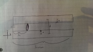
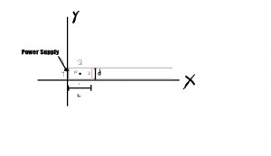
A rail gun is a simple assembly involving more complicated physics. It consists of a power supply connected to two parallel rails. Between these rails is a projectile that completes the circuit. The power supply (in this case we are modeling it as several capacitors) will release current into the circuit, instigating a number of forces which we will attempt to model. Below is a very generic

railgun

example of a rail gun circuit. Our original goal was to find the equations of motion for the railgun and hence functions for velocity and position. However, the mathematics required for this project has revealed itself to be immensely complicated, certainly much more so than we had expected. Many of the preliminary equations we find are based on the velocity itself, something we cannot know until the very end under our current plan. We have decided to go about it a different way, solving for all the relevant phenomena we had previously sought (current, b-field, emf) and using standard speeds of rail guns as constants to model said phenomena. In both our projects we will begin by deriving the most generic version of the magnetic field, caused by some current flowing through the circuit. This will require the Biot-Savart law:

(1)   \begin{equation*} B=\frac{\left(\mu _0I(t)\right)}{4\pi }\int \frac{dl\times r}{r^2}\) \end{equation*}

From Griffiths, the magnetic field at a point near a current carrying wire will be:

(2)   \begin{equation*} B=\frac{\left(\mu _0I\right)}{4\text{$\pi $z}}*\left(\sin \left(\theta _1\right)-\sin \left(\theta _2\right)\right) \end{equation*}

Here, the magnetic field at a point p is a superposition of the magnetic fields created by the four sections of the current carrying wire. B1 and B3 will be the fields of the two rails, B2 will be the field of the projectile, and B4 will be the field of the power source.

(3)   \begin{equation*} B_1=\frac{\mu _0I}{4\pi }\left(\frac{1}{y}\left(\frac{x}{\sqrt{x^2+y^2}}-\frac{(L-x)}{\sqrt{(L-x)^2+y^2}}\right)\right) \end{equation*}

(4)   \begin{equation*} B_2=\frac{\mu _0I}{4\pi }\left(\frac{1}{(L-x)}\left(\frac{y}{\sqrt{(L-x)^2+y^2}}-\frac{(d-y)}{\sqrt{(L-x)^2+(d-y)^2}}\right)\right) \end{equation*}

(5)   \begin{equation*} B_3=\frac{\mu _0I}{4\pi }\left(\frac{1}{(d-y)}\left(\frac{(L-x)}{\sqrt{(L-x)^2+(d-y)^2}}-\frac{x}{\sqrt{x^2+(d-y)^2}}\right)\right) \end{equation*}

(6)   \begin{equation*} B_4=\frac{\mu _0I}{4\pi }\left(\frac{1}{x}\left(\frac{(d-y)}{\sqrt{x^2+(d-y)^2}}-\frac{y}{\sqrt{x^2+y^2}}\right)\right) \end{equation*}

The total field, of course, would be the superposition of these four equations. However, after having done a good amount of research and going through trial and error, we have discovered that when the rails (L) are much longer than the projectile and power source (d), we only need include the effects of the rails. Below is this magnetic field:

(7)   \begin{equation*} B_{\text{tot}}=\frac{\mu _0I}{4\pi }\left(\left(\frac{1}{y}\left(\frac{x}{\sqrt{x^2+y^2}}-\frac{(L-x)}{\sqrt{(L-x)^2+y^2}}\right)\right)+\left(\frac{1}{(d-y)}\left(\frac{(L-x)}{\sqrt{(L-x)^2+(d-y)^2}}-\frac{x}{\sqrt{x^2+(d-y)^2}}\right)\right)\right) \end{equation*}

Now, to find the magnetic field upon the projectile itself, we substitute L for x and get:

(8)   \begin{equation*} B_{\text{proj}}=\frac{i \mu _0 \left(\frac{L}{y \sqrt{L^2+y^2}}-\frac{L}{(d-y) \sqrt{(d-y)^2+L^2}}\right)}{4 \pi } \end{equation*}

From here, it is my responsibility to find out how the rail gun acts as a circuit. There are a couple parameters that I have been able to establish pretty easily. The first is the resistance of the circuit as a whole. This resistance is:

(9)   \begin{equation*} R=\rho \frac{(2L+2d)}{A} \end{equation*}

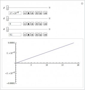
manipulate1

Where \rho is the resistivity and A is cross sectional area.

From there, we can start to look at the current created by the a capacitor with charge Q_0 and capacitance C discharging with the generic

(10)   \begin{equation*} I_{\text{cap}}=\frac{Q_0}{\text{RC}} \end{equation*}

By replacing the R term we found above,

(11)   \begin{equation*} I_{\text{discharge}}=\frac{Q_0}{\text{C$\rho $}\frac{(2L+2d)}{A}}e^{\frac{-t}{\rho \frac{(2L+2d)}{A}C}} \end{equation*}

We also know that this current is not the only current present in the circuit, as there is an induced current caused by the EMF created by the changing area and Magnetic Field (aka Magnetic Flux). We know that EMF ( \epsilon ) is equal to:

(12)   \begin{equation*} -\frac{\text{d$\phi $}}{\text{dt}}=\frac{\text{dB}}{\text{dt}}d\frac{(\text{dx})}{\text{dt}} \end{equation*}

We use the chain rule to say that:

(13)   \begin{equation*} \frac{\text{dB}}{\text{dt}}=\frac{\text{dB}}{\text{dL}}\frac{\text{dL}}{\text{dt}\\ } \end{equation*}

Where the second term

(14)   \begin{equation*} \frac{\text{dL}}{\text{dt}}=v \end{equation*}

Solving for the derivative of B with respect to L, I got that

(15)   \begin{equation*} \frac{\text{dB}}{\text{dL}}=\frac{i \mu _0 \left(\frac{\frac{1}{\sqrt{(d-y)^2+(L-x)^2}}-\frac{(L-x)^2}{\left((d-y)^2+(L-x)^2\right)^{3/2}}}{d-y}+\frac{\frac{(L-x)^2}{\left((L-x)^2+y^2\right)^{3/2}}-\frac{1}{\sqrt{(L-x)^2+y^2}}}{y}\right)}{4 \pi } \end{equation*}

It is after this step where it gets complicated. I have used this expression to solve for EMF and then current, but the results are far from elegant and I am going to withhold them until I can validate the methodology. From here, there are two options. Griffiths proposes that EMF simply equals this result times velocity. However, I think that I may have to integrate the magnetic field over the area of the loop. I have tried this and have not had luck; the integral has been equal to 0 every time I’ve tried, something I know to be false. Once I figure this out, I will be able to animate and model all of these expression, and collaborate with John to achieve our final result.

As for our physical model, we will work with Professor Magnes to find something safer and more practical in the context of Vassar.

References:

Griffiths, David J. Introduction to Electrodynamics. Upper Saddle River, NJ: Prentice Hall, 1999. Print.

http://webphysics.davidson.edu/physlet_resources/bu_semester2/c11_RC.html

https://physics.le.ac.uk/journals/index.php/pst/article/viewFile/468/275


Share

Project Plan: Rail Gun

Sources/Resources:

  1. Introduction to Electrodynamics by David J. Griffiths
  2. http://web.mit.edu/mouser/www/railgun/physics.html
  3. http://www.dtic.mil/dtic/tr/fulltext/u2/a345008.pdf
  4. https://physics.le.ac.uk/journals/index.php/pst/article/viewFile/468/275
  5. http://www.instructables.com/id/Rail-Gun-Linear-Accelerator/
  6. Vassar College Lab Technicians

Materials:

  1. LaTeX and Mathematica Software
  2. Pen and Paper for derivations
  3. Gas Reservoirs
  4. Gas Valves
  5. Steel Tube
  6. Pneumatic Pipes
  7. 10 400 Volts 450 uF Capacitors
  8. Solid Aluminum Bar
  9. Acrylic

General Project Plan:

The first and most important part of our project is to use Mathematica to model the magnetic fields, current, capacitance, and eventually forces/equations of motion of a generic rail gun. This will require a great deal of derivation using principles from Griffith’s book, and a working knowledge of Mathematica. We have found several resources online that will help us through the derivation process.

The rail gun will essentially be made of four components: a power supply, two rails, and a sliding bridge with a projectile attached. This bridge will complete the circuit. The current will create a magnetic field and push the projectile/bridge forward. This motion generates a number of interesting properties which we hope to model on Mathematica.

We will build a rail gun using materials both from the lab and that we acquire independently. After doing so, we will take a video of the rail gun using Vassar’s high speed camera. We then will use video analysis software like LoggerPro to analyze our results and compare them to known existing value and the values that we calculate.

Estimated Time Line:

Week 1 (4/6-4/12): Acquire working knowledge of Mathematica and begin hand derivations of relevant equations and concepts. Make list of materials required for assembly of railgun.

Some basic equations we will work with are:

Biot Savart-

(1)   \begin{equation*} B(t)=\frac{I(t)\mu_0}{4\pi}\int\frac{dl \times r}{r^2}\ \end{equation*}

Ampere’s Law-

(2)   \begin{equation*} \nabla \times B = \mu_0J + \mu_0\epsilon_0\frac{\partial E}{\partial t} \end{equation*}

Ohm’s Law-

(3)   \begin{equation*} I(t)R = V(t) - \varepsilon(t) \end{equation*}

Resistance-

(4)   \begin{equation*} R = \frac{\rho l}{A} \end{equation*}

I will apply these equations to our specific case and find how they change with time specific to the parameters.

Week 2 (4/13-4/19): Finish my models of current and resistance as functions of time. Begin to plot them on Mathematica. Attain all materials for assembly of rail gun

Week 3 (4/20-4/26): Finish modeling current, resistance, and capacitance on Mathematica. Combine my results with John’s results to model equations of motion. Finish assembly of rail gun

Week 4 (4/27-5/3): Test rail gun and compare results to our experiment. If time permits, factor different mediums/materials into the Mathematica models.

Collaborator:

I will be working with John Loree. He will use mathematica to model the induced magnetic field and forces upon the railgun. Together, we will build the railgun.

Share

Elias Kim Spring Project

Project Proposal:

Electrodynamics provides for some frighteningly fascinating applications. John Loree and I plan on investigating the physics of rail guns, powerful machines that fire slugs at high velocities using electromagnetic forces. We plan to build a functioning gun and analyze its motion with LoggerPro. Furthermore, I hope to use Mathematica to model the physics involved in the circuitry of the gun. This analysis will include finding current as a function of resistance, charging capacitors in the system, and the induced EMF. John and I will combine our results to produce general equations of motion for the rail gun.

Share