—-Project 4/27—-

I finally fixed my calculations. I was having trouble using Watts, dBw, and dBm. This meant that I was off on my  initial calculations by a factor of 10^-6 (alot I know, but still in the right ballpark).

This is totally cool, to me anyways. After playing around with all these numbers, I finally get the answer that looks right. The problem was with conversions of the power units. I was subtracting dBw from dBm or something like that. I blame the book I was using because it did not explain what dBm’s were. 2.15 dBm converts to 0.0016 watts, a much more realistic loss due to a small hill, and still overshadowed by free-space loss.

—-Project 4/26—-

I had more of a problem finding a suitable model to account for the terrain, than the actual mathematics of the model. After reading about the Egli Model, Longley–Rice model, an several others I landed on the ITU Terrain Model (Don’t worry, I didn’t use Wikipedia, its just the easiest to link to. And I’m going to steal their formulation images). This one seems to be the only that is within my reach. It is based on diffraction theory, taking into account the highest obstruction of the Fresnel Zone (Explained further down).

= Empirical Diffraction Loss. Unit: Decibel (dB)

= Normalized terrain clearance. Unit: None.

= The height difference. Unit: Meter (m)

= Height of the line-of-sight link. Unit: Meter (m)

= Height of the obstruction. Unit: Meter (m)

= Height of First Fresnel Zone. Unit: Meter (m)

= Distance of obstruction from one terminal. Unit: Meter (m)

= Distance of obstruction from the other terminal. Unit: Meter (m)

= Frequency of transmission. Unit: Megahertz (MHz)

= Distance from transmitter to receiver. Unit: Meter (m)

As you can see, it is quite accessible. The one term we did not touch on in class is the Fresnel Zone (again, Wikipedia is just easy to give quick explanations). Its basically a volume of the radiation pattern resulting from diffraction of the antenna. The more this space is infringed upon, the weaker the signal.

I could potentially apply this term for every radian, and get a 360 degree plot, however that would take way much more time pouring over topo graphs. Besides, my original objective was to model it just to Vassar.

So I went to the topo maps in the basement of the library. There I found a 500 foot hill, and a 2oo foot hill between us. Encouragingly, the rest was relativly flat. I plugged in the following values:

d=11666
f=91.3
ho=152.4
d1=4735
d2=6930
h=(320*d2)/d-ho
F1=17.3

A=10-(20*h)/F1

Incredibly low (free space loss was more)
A=2.15 dB

Subtracting this loss from my previous value: -30.62 dBm- 2.15 dBm=-32.77 dBm (0.528 microwatts)

—-Project 4/20—-

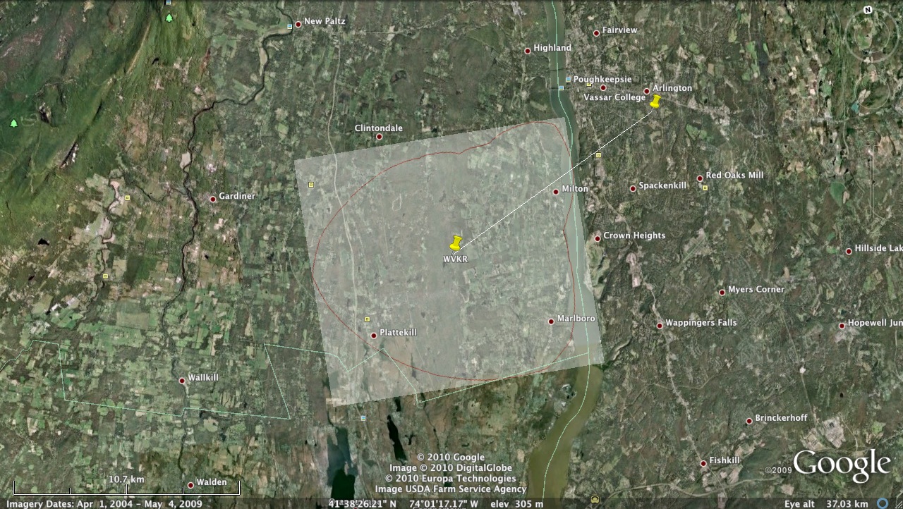
I decided to try to model WVKR’s radio reception, specifically here on Vassar Campus (the radio tower is southeast a few miles). I knew that this would by no means be very accurate. We all know wave interference can get quite messy, and change from day to day. Waves bouncing off low clouds, diffracting around buildings, interfering with other channels and such. Indeed, real life models are largely based on empirical equations. But the main idea is to project the amount of power delivered to our area. More power means better quality, and this is not digital (as far as I know), so the quality varies with the power delivered.

Map of the two points of interest.

The distance between the college and the station is approximately 7.24 mi (11.65 km) as the crow flies (FM signals are delivered as line-of-sight)

Unsurprisingly there are so many factors that computer models are largely necessary in order to process them all. I ran across a particularly well-designed freeware for Linux called SPLAT! where you can put in all the specifications of your antenna and it will process a coverage map taking into a majority of these parameters. Similarly, MIT has a website that provides a map of basic coverage for WVKR. I was happy to run into this one in particular because they base theirs on the same specifications that I will be using (though I have no idea what model they use).

Another area of interest is configuring the receiving antenna to accept the signal. Again there are many issues to consider, so for my purposes, I am going to assume that the power delivered is the power received.

So the FCC give me several key specifications about the WVKR tower. Luckily, they provide a important, measurement the ERP. The ERP (Effective Radiated Power) is a standard measurement (watts) of radio frequency energy. This term includes transmitter power output, transmission line attenuation, antenna directivity, and others. This is great because it takes care of all those nasty 1/r^2 terms when looking closely at the antenna. However, the power delivered also depends heavily on the height above average terrain (HAAT) which is perhaps more of a factor in the effective coverage. So I have the ERP (accounts for many gains and losses), HAAT, the height of the antenna, and frequency. The transmitted power and gains (for the most part) have been accounted for. Now I need to account for path losses from the antenna to the college. This is the biggest unknown.

A model of radio frequency propagation can start out quite simple, not very accurate of course, and get more complex as it gets more accurate.

The first loss, most basic loss, is free space loss. It depends on the frequency and the distance to the receiver.

 

In SI units, or:

 

Where f is measured in MHz, and the distance is measured in Km. Notice the logs. Since this equation is mainly used by engineers, they like to use the log scale, and hence loss is measured in dBs.

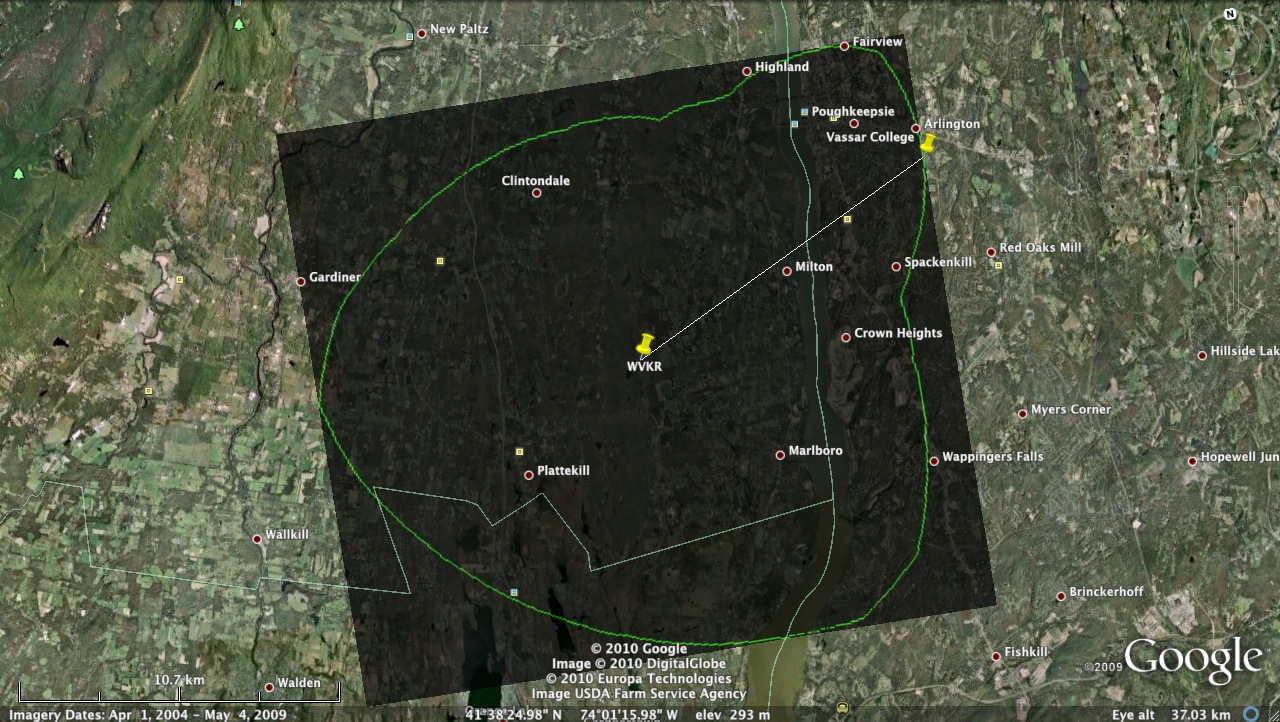
Now WVKR has coverage as linked to below.

Distance of 1.86mi – Power delivered 13.24 microwatts

Distance of 4.37mi – Power delivered 2.40 microwatts

Distance of 7.24mi (Vassar College)– Power delivered 0.87 microwatts (93.00 dB of loss)

Now it appears the this 0.87 watts is too weak to be useful. Indeed I beat my head about this for several, hours before actually considering the fact that radios, depending, can read power down to the nanowatts.

The next factor am trying to introduce is the terrain.

Mountains, buildings, and vegetation also contribute a lot. As FM frequencies are “line of sight”, a single mountain could potentially block all power. Or it could bring together in phase components of the signal and actually provide gain. Clearly, this is a difficult direction to go, so I am spending more time on it.

—-Project Proposal 3/23/—-

I would like to investigate how EM waves are transmitted by radio towers. Hopefully I can create a model of an antenna that will demonstrate the waves that are transmitted, depending on  its shape and the currents are applied. Then exploring several real-life antenna and describe how their configurations help their purpose. I am not sure what program draw this in though. Then if I can, I would like to take it farther and see if I can model the transmission of radio waves as they pass over over mountains or cities and such.

—-Journal Update 3/22/—-

My journal  is where I list any questions I have. I also list useful website I have used, or any that have been recommended to me. I haven’t yet, but I probably will use it to list notes for my project. Sometimes I also like to list the reasons why I like lists. If I have a good way of thinking about a topic or problem that makes it easier to understand, I’ll often write that in as well. I also have a running ranking system that I use to tell me which peers of mine usually do the homework first, best in-class notes, reading first, helping abilities/willingness ect.  for times when I may be in a pickle. That is all I use it for. Nothing in it as a study guide (that’s here), and I did not use it to decide on a project.

I also use it as scratch paper a lot

—-Homework—-

The best wave animation on the blog site.

The 4.10 vector field

The dielectric snells here. Notice how there is no total internal reflection

—-Refrence—-

I really do not want to post guidelines to homework, because I would probably be wrong, and I don’t really have feelings to write down. So I decided to take advantage of our ability to edit each others posts, and turn mine into a sort of wiki page. A wiki page of useful equations and relationships, and centrally located equations. I’ll get us started:

Equations from Book/Definitions	Equations from Problems/Sample Problems	Useful rules of thumb
σb=P·n.

ρ_b=-(divergence) P.Electric field of a capacitor: E=σ/ε₀.

Uniformly polarized sphere radius=R     E=-1/(3ε_o)P for r<R .

Sphere with P(r)=kr                         E=-kr/ ε_o r<R          E=o  r>R .

A sphere of homogenous linear dielectric is placed in an otherwise unifrom electric field E_o. E inside sphere is unifrom = 3E_o/(ε_r+2).When P is uniform, ρ_b=0 .

D is parallel to E in a vacuum.

and if no one else uses it, at least I will.

—-Nonsense—-

A mosquito taken down by a laser. Watch