
In this project, I focused on creating a program which would model the motion of any system of any number of objects interacting gravitationally. I used this project as a way to become more comfortable with computational methods we’ve already explored in class, to expand upon them, and to become more comfortable with the actual modeling and animation process, so that I can become more skilled in presenting the information I gather computationally. I was also attracted to this subject matter, because the generalized form I developed it for allows me to learn something new every time I plot it, exploring new systems every time.
Background
The “N-body problem” is one that has plagued physicists since Newton’s times. Newtonian/Classical gravity is defined by  The behavior of two objects, interacting through Newtonian gravity, is well understood, easy to analyze by hand, and easy to model. However, as we increase the number of objects in our system, the problem immediately becomes far more complicated. People have studied the n-body problem for centuries, searching for a solution. In the late 19th century, the king of Sweden offered a prize to anyone who could find a general solution to the n-body problem. This challenge was left unmet, and the award went to Poincaré for an unrelated accomplishment. In more recent times, understanding the n-body problem has become far more feasible with technological advancements and the associated rise of computational physics. While there is no analytical solution to the n-body problem for 3 or more bodies, we can use computational methods to model and better understand gravitational interactions between celestial bodies and their resulting behavior.
We begin this analysis of gravitational interactions using the formula for gravitational force in conjunction with Newton’s Second Law.
From this, we get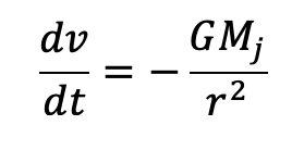 To analyze this behavior, we must examine the system component by component. This results in the rate of change for velocity
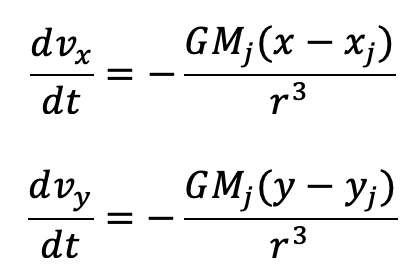
This velocity rate of changes allow us to analyze the position of all of the celestial bodies in our system, since
Method
Equations of Motion
To model the n-body problem, I start by creating a set of input variables. This allows to me to create a very general program which should run whether we examine a system of 1 celestial body, 10, or 100. The program allows the input of number of bodies in the system, mass, initial position, initial speed, and initial direction of motion for each body.

This is the code for collecting information from the user of the program. This excerpt of code applies to all objects other than the first.
Once the inputs have been obtained, we can proceed with the Euler-Cromer method to analyze the motions of however many bodies.
The Euler-Cromer method uses a known rate of change for some desired variable, and adds the product of the rate of change with some step of the independent variable, to approximate some behavior. The distinction between the Euler-Cromer and Euler methods lies the fact that Euler-Cromer uses a newly calculated rate of change to calculate the new position. The Euler-Cromer method is effective for 2nd order differential equations, such as this case, where the Euler method fails. In the case of the n-body problem, this method takes the following form: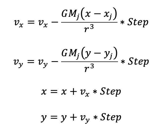
However, the above form only accounts for an object interacting with one other object. To address this, I summed the acceleration due to each object in my code.
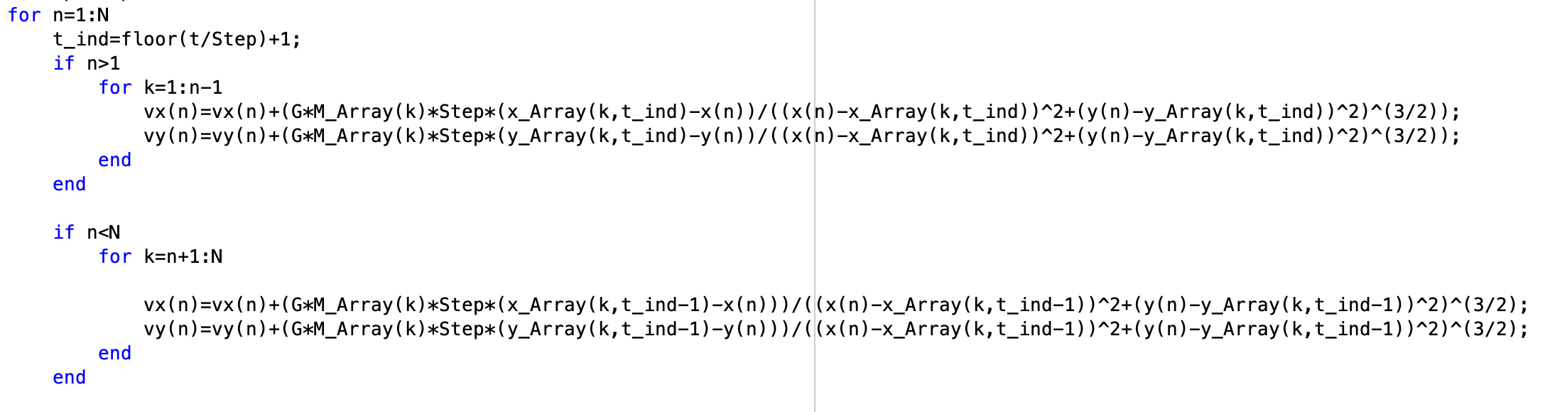
This excerpt of code includes the summation of the gravitational forces and their influence on each object’s velocity.
Plotting/Animation
To understand how these interacting bodies behave, I examined their motion through graphing their paths and animating their motion. This plots demanded very little in terms of new plotting/animation methods, but rather demanded a lot of finessing, not all of which paid off. The drawnow command in conjunction with “hold on” and “hold off” produced the animation plots, whereas the same command only with “hold on” provided the plotted paths.
This is the code which plots the path of each object as we cycle through each time step.
Here is the code which plots the animation of each object’s motion. The primary difference between this code excerpt than the previous one is the use of “hold off”.
Results
It is hard to comprehensively discuss the results of this program because its input-based nature leaves infinite potential results. To examine how systems of n number of celestial bodies behave, I will discuss several cases as n increases.
Case 1:
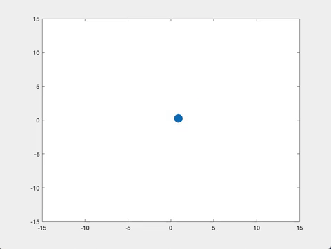
This case is the most simple and best understood in case, in which two bodies interact gravitationally. The initial conditions of this case are as follows:

Graphing the path of each of these objects yields the following result:
Above is the path of each individual object in Case 1, on a plot in units AU.
This (messy) version of the previous plot is simply to provide clarity for each individual path of the objects.
Below is a clip of the animation for this case.
This is a 15 second clip of the animation of this case’s behavior. I could not include the entire animation because the video would not work, and GIFs are limited in length. If the animation is not playing automatically, click to view.
The results for Case 1 are precisely what one would expect from such a case. Object 1, the more massive object, experiences smaller acceleration due to the gravitational force from Object 2 than vice-versa, yielding a much smaller spiral of motion.
Case 2:
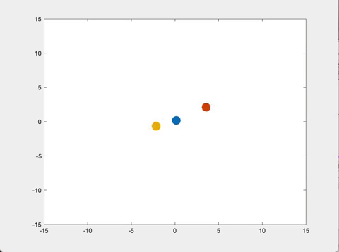
Maintaining the same conditions for the first two objects, we then consider adding a third into the system and see how it impacts the motion of the objects within the system. The initial conditions are as follows: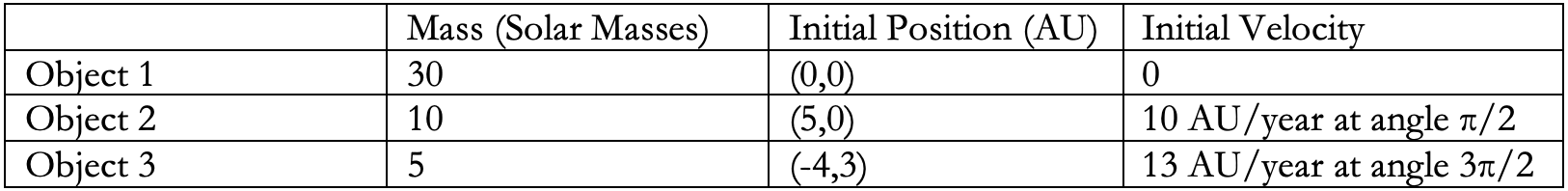
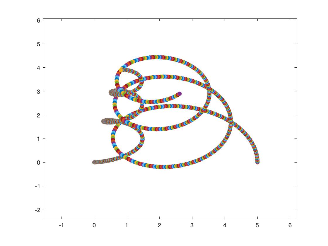
The results of Case 2 are graphed below.
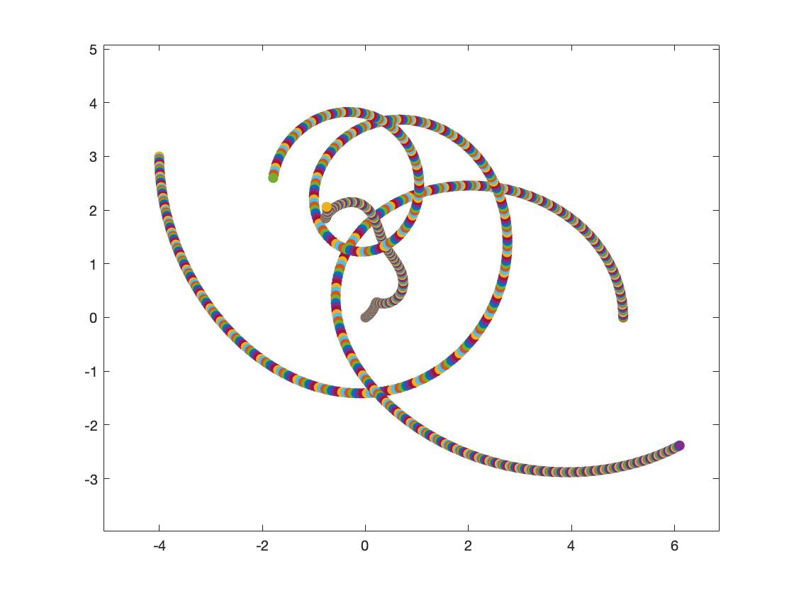
The paths of gravitationally interacting objects 1,2, and 3 are shown above, on a graph of units AU.

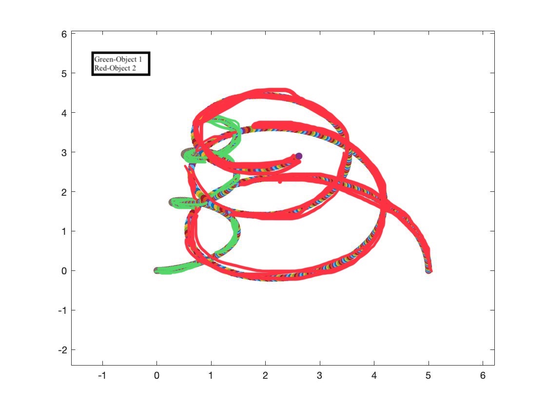
This graph is simply the plot above, with sketched color coding to clarify the paths of individual objects.
An animation of this case is shown below:
This GIF is 15 second clip of the animation of Case 2. If not playing automatically, click to view.
Case 2’s results are less predictable than the results of Case 1, because of the additional object included. The most massive object (Object 1) still changes position the least, with each object of a lower mass moving more significantly than the last. This is the first case whose results we could not have calculated analytically. We can understand the trajectory of an object influenced by more than one object if one or more of those objects are held still, but the fact that each and every object experiences a gravitational force due to every other object eliminates the possibility of an analytical solution.
Case 3:
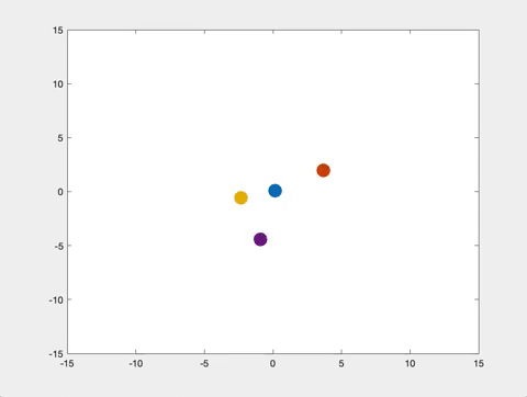
Adding a fourth body to our system, we will further examine how motion evolves as n increases. The initial conditions of this case are listed below. 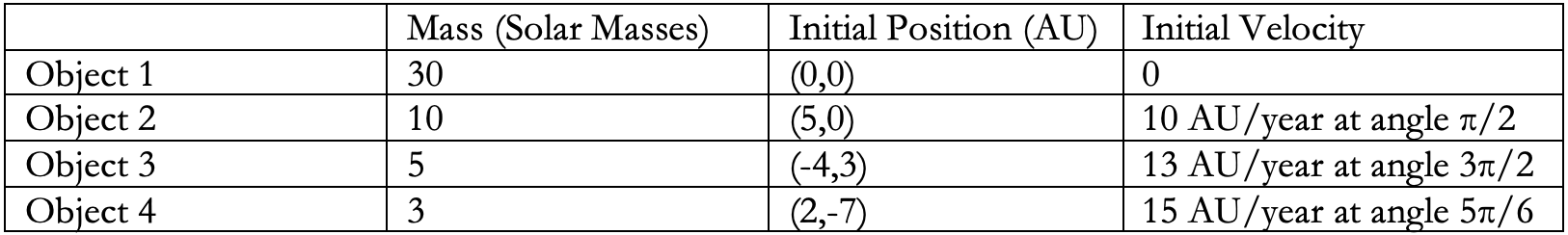
This case yields the following results:
On a plot with axis units AU, objects 1,2,3, and 4’s paths are shown.
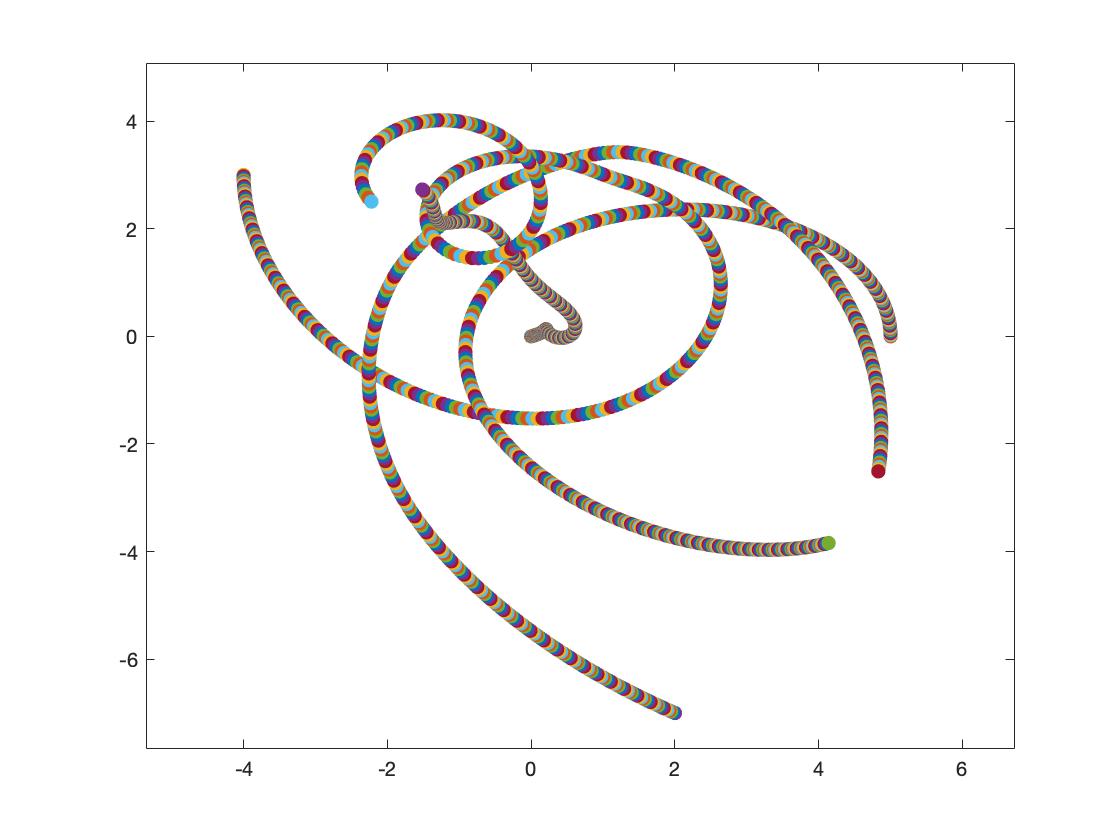
The same plot as above is shown here with sketched on color-coding the clarify the paths of each individual object.
The animation for this case is shown below.
This GIF is a 15 second excerpt of the animation of Case 3. If it does not play automatically, click to view.
This case further demonstrates the transition from order in a two body system, to a far less ordered and less predictable system as n increases. Where in Case 1, object 1 moved in a clear spiral, here object 1 moves in a slow and oddly-shaped motion, as the forces it experiences are now based on the motion of 3 different objects.
From here we could continue to add more and more cases as n increases to watch this shift more clearly. However, while this program is theoretically general, and can run more than 4 objects at a time, as n increases, the program’s effectiveness decreases. The limitations and flaws in this program become and more likely to obstruct results, the more objects we consider in a system. I will discuss these flaws and the next steps to take to correct them below.
Obstacles/Limitations
- 2-D
The first limitation in this program is that it views celestial motion as 2 dimensional, where our universe is clearly exists within (at least) 3 dimensions. I made this choice to examine orbits and celestial motion from the perspective we usually view it ( we often view orbits as 2 dimensional, where they are not entirely), despite the fact that it does not entirely match reality. - Collisions
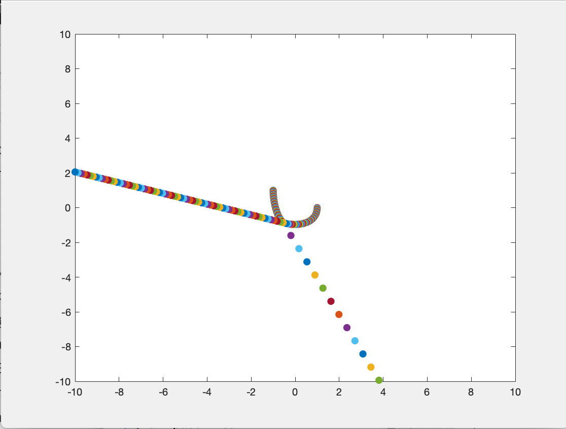
One problem within this program is that it is not built to address collisions of celestial objects. When two objects wind up in the same position in the program– something that is physically impossible, but which this code does not explicitly prevent– they experience some large acceleration away from the other object. This behavior is not physically accurate and is a result of Matlab’s inability to understand an infinite acceleration.Here is an example of what a plot looks like when two objects collide:
This plot (with axis unit AU) shows the way that objects react when they collide in this program. Both objects can be seen bolting away from one another immediately after their collision.
- Inaccurate Plotted Points
This is an issue that has not occurred often, but for which I have little explanation. Occasionally, in the middle of a program running, a new path of an unknown object will begin being plotted, which appears to be fairly massive, because it attracts the surrounding objects fairly strongly. - Path Plotting: Rainbow Everywhere
As illustrated by my attempts to color-code my path plots, I have not yet found a way to plot the path of n number of objects in a for loop, where the program recognizes the paths of each object as distinct. This is why my original plots are all comprised of many colorful points, instead of a consistent color for each object. This problem also makes diagnosing the cause of the previous issue, because I cannot see which object the program is recognizing as also being in a different position. - Flashing Animation
Assuming the links to the animations work properly, you can see that all objects except Object 1 are flashing. Having experimented with draw now, refresh data, hold on, and hold off, I have not yet identified a way to have a consistent, non-flashing animation of these systems’ behavior.
Where Next?
- 3 dimensional
Making this program 3-dimensional would be fairly simple upgrade to the program, to understand gravitational interactions as they actually occur in our universe. This would simply demand obtaining input information about the z component of motion, and applying it using the Euler Cromer method. - Conservation of Momentum
Taking into account conservation of momentum would be one way to potentially address the limitation in my program in regards to collisions. Without significantly more information, this would likely demand the assumption of inelastic collisions in all cases. I could achieve this by adding the masses of colliding objects in one objects’ array information, and setting the other objects’ mass to zero. This however, may not actually be a large upgrade in terms of accuracy, as perfectly inelastic collisions are no where near the reality of what occurs when objects collide in space, so it would have its drawbacks as well. - Individual Track Paths of Different Objects
Another clear next step would be to solve my issues in plotting, and develop a method where the program would recognize the individual paths of different objects, instead of considering every data point as unique. I admittedly am not sure how to accomplish this. However, once this is accomplished, it would play significant role in finding the error which causes random data points to pop up where they do not belong (problem #3 above). - Somehow Stop Flashing???
The other significant next step in developing this program would be to solve the issue of flashing objects. This would likely just require even more deep diving on the internet into MatLab animation techniques, however the particular solution to this problem evaded me for the duration of the project length.
Another step moving forward that I would take with this program is to explore more explicitly what yields a stable (or stable-enough) orbit so that I could examine the behavior within a system of objects for a longer period of time. In this case, I would also explore more of the physics of the system, seeing how different objects’ velocities change with respect to time, how their acceleration changes, etcetera. With the program as it stands, exploring those would likely yield a fairly confusing set of graphs, with objects’ behaviors layered on top of each other in an incomprehensible mess. However, if I were to take the time to find systems for which this information is notable and readable, and sort through how to represent it sensibly, this would provide a lot more context for the behavior of these systems.
