
My final project for Computational Physics was selected based on the interest of exploring systems within thermodynamics, particularly gas/liquid behavior through different mediums. Conveniently, the textbook used in this course had an entire chapter devoted to several types of Random Systems, particularly one involving modeling diffusion using the cream in coffee concept. Although I aimed to complete 2 separate codes for my final presentation, instead I developed 3 different versions of a code that modeled the spread of cream particles in coffee over a certain period of time. However, before jumping into the specifics of that code, let’s explore some background information.
What is Diffusion?
To briefly review from our unit on Random Systems, diffusion is a process resulting from the random motion of particles where the net flow of matter goes from a high region of concentration to a low region of concentration. In simple terms, diffusion is the transport of materials. Let’s look below at a diagram depicting this process.
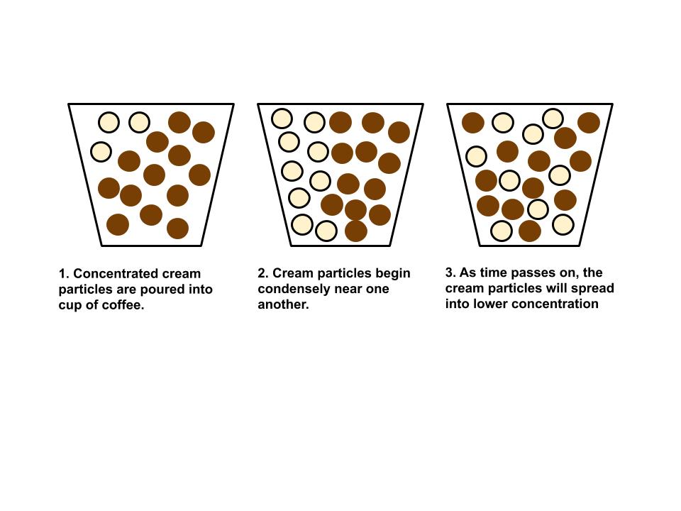
Above is a 2D view of Diffusion inside of a Coffee Cup with Cream
Tentative Plan for Project (3 Components)
Part I – Diffusion in 1D through Density Equation(s)
To begin, I decided to look into how the density is dependent on changes to time and displacement. With those concepts in mind, the textbook introduced the equation of density as:
Spread of particles over time can be described through this density equation when coded in.
The equation describes a random walker, which can be thought of as a particle. Initially, this walker will start at some origin point, if there are multiple walkers, they will also begin at this specified location. At t=0, the density of these particles will be concentrated at this origin point and they will not have displaced themselves until after more time elapses. According to the book, we can verify this displacement and density as we go through several iterations using the following equation:
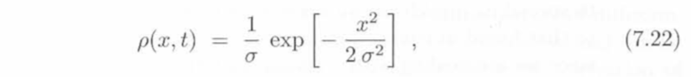
This function is crucial because it illustrates this dependence of the diffusion constant on time, where σ =√ 2Dt.
As simple as this code is, it was challenging because three different parameters were changing simultaneously. I had to create two arrays of time and displacement that needed to be the same length in order to loop through the density equation. Nonetheless, the error of this code lies in with how the density equation is either written because only t=0 can plot in the code, which just appears as a straight line. This makes sense because all the density will be condensed at x=0. For that reason, I decided to focus in all my efforts to perfecting my second code that would be able to plot cream particles displaced over time. However, here is the code that still needs to be revised to run properly.
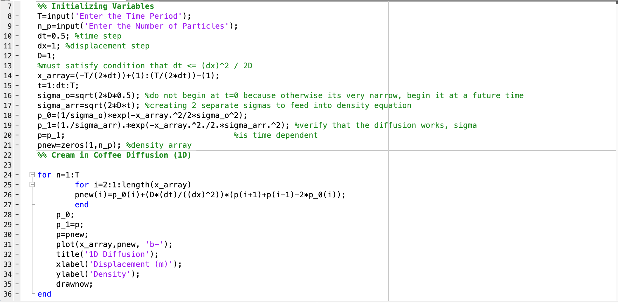
Despite this code not working, it had a lot of good direction and it did add to my understanding for developing my second code that I submitted for this project.
Part II – Cream Particles in a Square Coffee Cup
In this part of the project, I attempted to recreate Figures 7.13 and 7.14 within Chapter 7 (pp 202). This simulation would be utilizing the computational method of a 2D random walk, which we did more recently towards the end of the semester. In this simulation, we assume at t=0, the cream particles are restricted to a box of specified dimensions. There were several noticeable characteristics from both figures:
- It was hard coded for those particles to begin in a box of 10 x 10 dimensions.
- Particles were allowed to overlap one another.
- Particles could not move outside the boundaries of this square cup (they should not move past the walls).
I wanted my program to be as user friendly as possible (also just somewhat unique from what the authors did), so I made input conditions that would let the user specify the dimensions of the box where the particles started, how big the overall cup could be (by using the idea of a grid layout), and restricting the particles from moving into a position that is already occupied by a particle (no overlapping). The final product of this code was developed into three distinct versions, the last one being my favorite.
Version 1 – Box of Particles Code
Since I had not practiced making functions in MATLAB within the course so far, I decided it would be good to utilize the benefits of using them for this simulation. It is not difficult to make a series of for loops to accomplish what this code does, but the code would condense in length with the usage of functions. The two primary functions in my code were: buildGrid and moveParticle, each of them served a purpose. buildGrid would construct the initial box that the particles would be restricted to and center them at the origin of the grid. We can imagine the buildGrid function creating a cup that is just an array of 0s and this initial position of the particles inside this box will be a series of 1s. moveParticle utilized cases rather than if else statements, which implemented the random walk portion of the code. I only allowed my particles to move in the +/- x and y directions, this could be modified to allow only diagonal directions, but beginning with this was sufficient for me. As the particles moved through different parts of this grid of 0s, these new locations would be marked with 1s. This first version did not allow particles to overlap and although the code accounted for that, the particles after several iterations would begin to drift to the right side of the cup rather than disperse evenly in all directions.
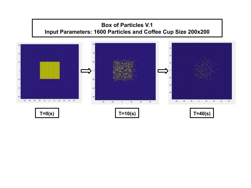
This version of code demonstrates how cream particles move throughout the medium of coffee overtime but they appear to drift to the upper right corner. This error could be in the buildGrid or for loop of the code.
Version 2 – Box of Particles Code
Going back to square one, I decided to allow the particles to overlap but again, however we lose too much information about the particles final location because many will end up moving into spots occupied by other particles. Nonetheless, it was important to revert back to this code because the particles do not displace towards the upper right portion of the square coffee cup.
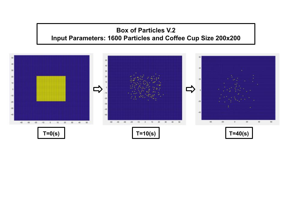
In this version of the code, the cream particles evenly disperse in all directions but so much overlapping takes place even after only 10 iterations. Again, we must correct for this.
Version 3 – Box of Particles Code
At last, I finally figured out how to correct this code! I decided that instead of restricting this system to just binary 0s and 1s, we can get positions of particles that could be 2s, 3s, and 4s. By doing this, we could tell where particles are overlapping with one another and see this position because a gradient effect would occur on the grid. When calling the grid into the command window, the user can see where particles are overlapping depending on the value at certain positions in the array. Nonetheless, when running the program, the lighter blue and green tiles are particles in their own unique position whereas yellow and orange tiles are particles that are occupying the same location as other ones. This program also made it easier to tell how the particles have moved.
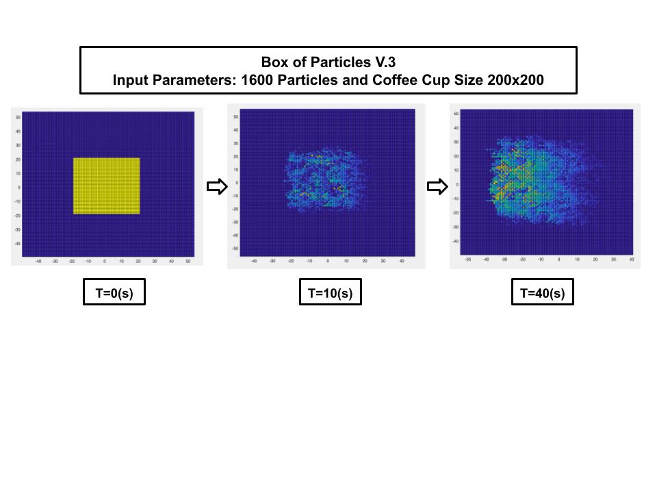
This final version of code would be the best to utilize so that all the cream particles can be somewhat distinguishable. The downfall to this code is that the different shades of tiles could make it more confusing to track individual particles.
Overall, all versions of the code could be useful for simulating different aspects of this scenario , but ultimately the third version would most likely be ideal to continue adding onto. If I were granted more time, I would have expanded this into a 3D simulation, which would have not been too complicated other than adding in z-dimension directions and making the initial grid system 3-D across. Also, if I had the chance to continue to work, I would have included values for entropy over time inside this simulation too. We would want to think about this as physicists because it is a value produced from this type of system we would want to study.
Part III – Experimental Simulation of Cream Particle Behavior in a Square Coffee Cup
Due to the fact I hit a roadblock with my first program, I decided to do a LIVE, experimental portion of this project. Here were the materials I used (+ thank you to Sara Ratliff who assisted me in conducting it):
- Bowl (used a square one here purposely)
- Food Coloring
- Timer
- Ruler
- Camera (iPhone 7 used here)
By using the software LoggerPro, I was able to insert a video where I used a square bowl of water in order to show how a drop of food coloring would diffuse over time. This experiment was not as simple as it seems, I had to put just a small amount of water in this square tupperware because otherwise the food coloring would not disperse in the x and y direction as much. To reiterate, I wanted to keep this as 2D, so with more depth of water in the container, the easier it was for the food coloring to sink rather than spread. Another feature I did not consider was the density of the food coloring itself, which did affect the time it took for it to diffuse throughout the water. Video file was too big to upload directly into blogpost so follow the link below to see the experiment happening.
Using this marker function inside LoggerPro, it had measured: the x and y position relative to the starting point the drop began (using the scale of the ruler placed above the square bowl) and the x and y velocity according to how much the drop moved as frames of the clip passed.

The blue dots represent where I marked the position of the food coloring drop and how it had moved as time passed. On the left side of this image, this the table automatically produced from this blue dots by LoggerPro.
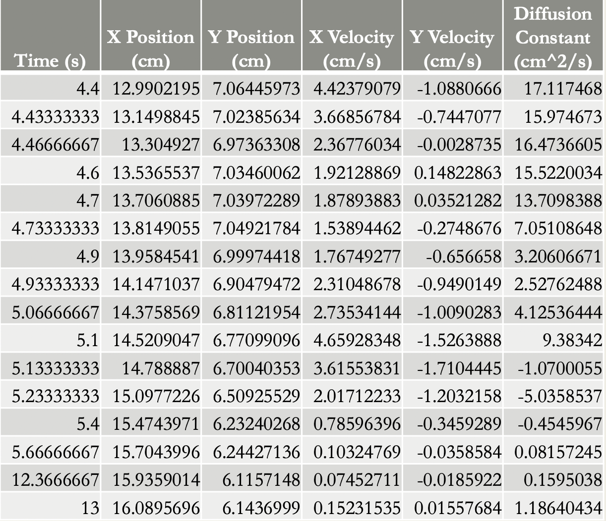
The diffusion constant computed for different times does vary too much that the final value found for the average D is most likely not that accurate but as with any experiment, some error is expected.
By tagging the location of the food dye, I compiled enough measurements to solve for the diffusion constant. Using the formula of:

I found the average diffusion constant for the experiment to be 6.427 cm^2/s.
Conclusions & Final Thoughts
Modeling random behavior is a challenge because every time I ran my program the results could be different each time. I thoroughly enjoyed struggling through the code because I did end up being able to present a program that could be effective in demonstrating diffusion in a computational way. If I were to repeat this project, I would have explored Brownian motion, which is diffusion but there is a component of the particles that have a large enough kinetic energy that they move and collide with one another. I would have accounted for those different collisions of particles and it would have tied to more of the original idea of my project which was about heat transfer. Otherwise, with the current code I have, as mentioned earlier, I would make my Box of Particles Code 3D and also maybe choose diagonal x and y directions instead. Plus, using the path those particles take, I would have also wanted to make a graph that described the entropy in the system as time went on.
