
By Jay Chittidi (’19), Lab Partner: Ellis Thompson (’20)
“Spooky Action at a Distance” is among one of the phrases that comes to mind for even someone without any experience with quantum mechanics thinks about some of the “paradoxes” of our quantum reality. It’s a phrase coined by Einstein when lecturing about quantum entanglement, and it was a phrase that came to my mind throughout our quantum mechanics class and the project I worked on with Ellis Thompson. We are fortunate to have a lab setup here at Vassar that allows students like ourselves to experiment with quantum entanglement and take real data that can (hopefully) reproduce the quantum mechanical conclusion that Bell’s Inequality does not hold (more on this later).
Warming Up to Entanglement
The critical idea behind entanglement relates to superposition. In class, we have worked a little bit with the idea that particles can exist as a superposition of states, thus involving multiple wavefunctions. For entanglement, two photons can exist in a superposition of the same state, such that a measurement of a property of one is dependent on the other (their wavefunctions collapse to the same state at the same time when observing one of them). In our case, the observable is the polarization state; the down-converted photons are in a superposition of vertical and horizontal polarization. Here’s the punchline — correlated photons will collapse to identical polarizations that we can detect. We call the detected correlated photons our “coincidences.”
The biggest takeaway should be this — the two photons aren’t “communicating” in any way. As one can imagine, if we have two entangled photons on opposite ends of the universe, a measurement of one will determine the state of the other. If the measured photon somehow sent information to it’s entangled partner, that information would have to travel faster than the speed of light in order for instantaneous collapse to occur! Instead, the nature of quantum mechanics is such that they two photons are said to interact “non-locally,” meaning that “communication” isn’t what’s happening here, but a purely quantum phenomena that both doesn’t fit our human understanding of interaction and (thankfully) doesn’t violate relativity.
So what about Bell’s Inequality? To explain that, we need to first consider the consequences of quantum entanglement. If we consider entangled photons at a very large distance apart, we might wonder how it’s possible for the entangled photons to I’ll go over the mathematics description of this briefly (it’s a complicated derivation and outside of the scope of our class). The Clauser, Horne, Shimony, and Hotle (CHSH) version of Bell’s Inequality2 applies directly to our own work in that we can substitute for polarization angles and determine whether our own data support or violate the theory of hidden variables to explain quantum entanglement. We can describe our data as follows with the “arbitrarily” defined variable for correlated photons under hidden variable theory:
1.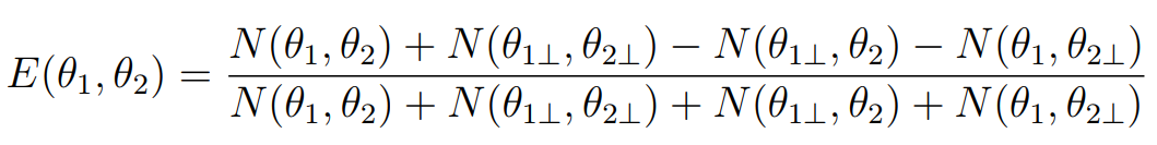
Here, E is a mathematical description of correlated photons and N is the number of coincidences as a function of the two polarization angles over a given time step. θ1 and θ2 represent the initial polarization angle for each detector, and θ1⊥ and θ2⊥ are θ1 + 90° and θ2 + 90°. As is evident, we expect that the number of coincidences to be a function of polarization! Then, we consider CHSH Inequality in the following form:
2. ![]()
The variable S is a function of E, which we obtain directly from our data. θ1‘ and θ2‘ are θ1+45° and θ2+45°. The final piece of our work is to say for all hidden variable theories, S ≤ 2. From our data, we hoped to demonstrate that S > 2 and thus that Bell’s Inequality doesn’t hold. The derivation of these equations and extremely complicated and nontrivial, and really just mathematical motions for understanding hidden variables, and thus is outside of the scope of our work.
Our Experimental Setup and More Background
I find that learning about entanglement in the context of our experiment specifically is most insightful. First, we use a violet laser (405 nm) that is intercepted by a half-wave plate that we set to 22.5° (leading to a 45° polarization). Then, we use a quartz plate to phase correct the light before it encounters the paired BBO crystal. Now here is where the “magic” happens. The non-linearity of the paired crystal results in some photons experience (random, probabilistic) phenomenon known as spontaneous parametric down-conversion (SPDC, like ACDC!), wherein one photon emerges from the process as two photons with twice the wavelength (infrared!).
Now, these down-converted photons obey conservation of momentum, and so they both form the same angle with the original beam path. The critical consequence of the conservation of angular momentum is that the polarization of the two photons are orthogonal to the “parent” photon. Further, the emerging photons have a polarization state (either horizontal or vertical) determined by the crystal pair, but we cannot know which crystal specifically results in the polarization state. This results in the two photons existing in a superposition of polarizations until at least one of them is measured. But, the consequences of the SPDC process mean that the same wavefunction describes both photons and thus a measurement of one causes the other photon to collapse into the same state. Hence, this sense of superposition is more than our traditional sense, as the two photons are entangled and correlated.
3.![]()
Equation 3, from Dehlinger and Mitchell1, represents the state of photons before they are down-converted. θl represents the angle from the half-wave plate and Φl is the phase shift from the quartz plate. The p subscript denotes that the polarization is from the pump beam.
4.![]()
Equation 4, also from Dehlinger and Mitchell1, is the state after down-conversion. The subscripts s and i represent the signal (detected) photon and the idler photon. I show these equations simply to demonstrate how after down-conversion, we cannot describe the state of either the signal or idler without considering the other. I point the reader to Ellis’s blog post for more about polarization states in the context of our quantum class, as she uses the Hermitian operator for a quick analysis of the formalism involved.
The down-converted photons actually emerge as a cone of infrared light we can detect (see Figure 3), but this also means that the coincident photons are all 180° from each other on the cone! This proved troublesome in our efforts and I’ll mention more later. Before the final leg of their journey, the (hopefully) entangled photons encounter a second half-wave plate, and then a polarizer that is the dependent variable in our experiment. Finally, the photons pass through an infrared filter we use to shield from ambient lighting, and then they reach our photo diode (the detector).

Figure 1: A bird’s eye view of the stage. See above for a detailed description

Figure 2: The detector assembly. Detector B is on an XYZ Transform to aid in alignment. See below for more details.
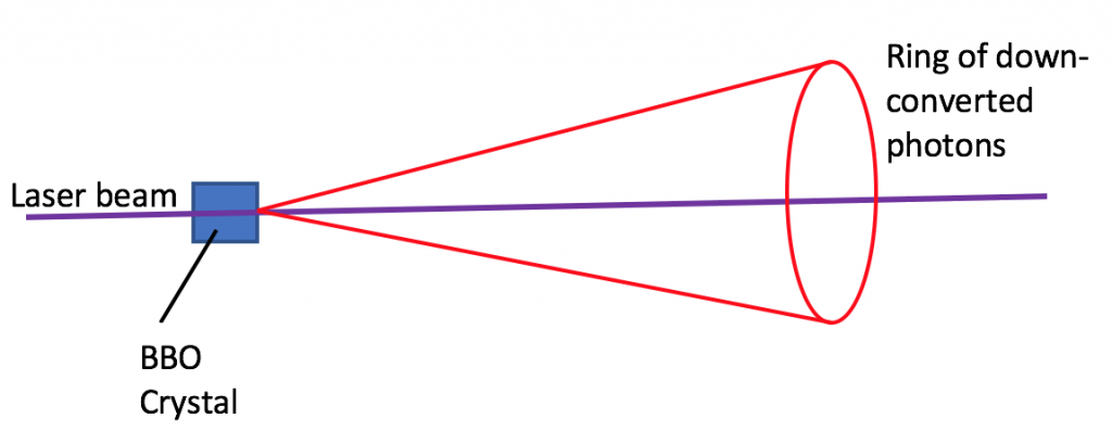 Figure 3: A diagram in a semi-2D plane of the ring of down-converted photons. Note that the purple beam is exactly in the center of the cone.

Our Struggles
At the beginning of our work, Detector B was quite misaligned. The cone of down-converted photons form a very thin stream, so exploring the parameter space with the detector was a very lengthy and tiresome process. Fortunately, we had the assistance of an XYZ Transform and Professors Daly and Magnes. In December, with a stroke of luck we managed to bring the detector close to alignment by adjusting the angle of the detector while exploring along the y and z axes.
Next, we made many fine adjustments to maximize the number of counts reaching Detector B. We were very systematic with this step, as we were able to realize where on the “circle” of photons we were by observing how the counts reaching the detector changed along the z and y axes. As is evident, laser alignment took the longest time for us!
Our next step was to maximize coincidences, which are not necessarily directly increased by placing our detectors where the down-converted photons are. We realigned the polarizer and half-wave plate in front of Detector B and locked them down, and this improved our number of coincidences significantly. The quartz plate, as mentioned earlier, adjusts the phase of the beam before down-conversion, and so at the suggestion of Professor Daly, we slightly rotated the plate until we maximized coincidences. With this final adjustment, we were finally ready to take data during study break!
Data
Looking closely at equations 1 and 2 will show that in order to calculate S, we need to measure the coincidences at 16 combinations of polarizations. We will refer to θ1 and θ2 as θA and θB and α and β as these are the formalisms adopted in Dehlinger et al. 20021. We choose to do this systematically where we fixed θA and went through the angles of θB, and rinsed and repeated. Our integration time was 10 seconds, a value that was twice that of which previous students used, but not inappropriate for our work, as saturation and other effects were not present, so we could increase our signal-to-noise. We plot the data in Table 1.
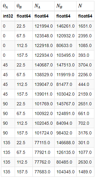 Table 1: A data table resulting from processing our work using Python (and the package Astropy). θA and θB are the polarizer angles for Detectors A and B, respectively. NA and NB are the total counts in each detector over the 10 second period, and N is the number of the counts that were coincidences.
We expect that for any fixed value of θA or θB, the resulting four measurements of coincidences should be describable by a sinusoid due to the relationship of orthogonality of the states (we expect minima and maxima). Unfortunately, our data do not reflect this as Figure 4 will show.
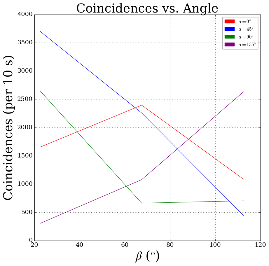 Figure 4: We plot the number of coincidences as a function of the polarizer angle for Detector B, while holding constant α (we choose to reflect the four values of α with colors). As is apparent, only for α = 0° does our data appear sinusoidal. What we expected were two minima and two maxima for each set of four measurements.
Results
The clear absence of sinusoidal behavior in Figure 4 is a sign that something isn’t quite right. To make this clear, however, we calculate S as described in equations 1 and 2. We report that from our data, we find S = -0.047 ± 0.028, which falls within the prediction of Bell’s Inequality. In other words, our results do not disprove Bell’s Inequality allowing us to rule out any local hidden variable theory. We determined our uncertainty simply using propagation of uncertainties through equations 1 and 2, and with the fact that the uncertainty on any individual measurement of coincidences is Poisson distributed. The data presented are the second round of data we worked with after the first also had a negative result.
Conclusions
Our results unfortunately do not reflect what we had hoped to prove, but we will note that many others have replicated this experiment and found quite the opposite, so our quantum reality is quite safe! We attribute our result to continuing troubles with our assembly. Specifically, we suspect that we may not have our detectors placed 180° apart on the cone of down-converted photons. We also were very careful not to mess with Detector A, as it’s wiring is quite fragile and sensitive, and because it lacked an XYZ Transform. It may in fact not be perfectly aligned with the cone of photons, leading to our incorrect result. If we had more time (perhaps the length of an independent project), Ellis and I are confident we would have been able to correct the setup and obtain better data.
However, as I hope this blog post emphasizes, Ellis and I have made huge strides in understanding quantum entanglement. I say “strides” because it is certainly not an easy topic to comprehend, and we have had many, many “Aha!” moments, only to find that we would then face more questions than answers. Importantly, we also made tremendous progress in bringing the experiment to a point where any lab student would be able to walk in, spend an hour understanding the setup, a half hour taking data, and be finished. While alignment is still an issue, we are quite close as is reflected by the significant coincidences and counts. Professor Sheung expressed interest in also helping correct the setup with me next semester, and I hope to do so in time for Ellis to run the show next year!
Acknowledgements
I’d like to thank Professors Magnes and Daly for suggesting the project and supporting us with tools, ideas, and encouragement throughout the stages of the project. Thank you to Professor Sheung for asking us to explain our project and then walking us through what might be going wrong with our data. Finally, a special heartfelt thank you to my partner in crime, Ellis “Barbara” Thompson, without whom this experiment would be nowhere and quite a boring experience.
References
[1] Dehlinger, Dietrich and Mitchell, M.W. “Entangled photons, nonlocality and Bell inequalities in the undergraduate laboratory.” American Journal of Physics 70, 903 (2002).
[2] John F. Clauser, Michael A. Horne, Abner Shimony, and Richard A. Holt. “Proposed Experiment to Test Local Hidden-Variable Theories” Physics Review Letters 23, 880 (1969).
[3] Galvez, Enrique J. “Correlated Photon Experiments for Undergraduate Labs” Colgate University (2010).
