In this project, I (and partner Jay Chittidi) investigate the concept of quantum entanglement in an experimental context. I will show how entanglement not only relates to the concept of superposition but also how it furthers our understanding of the differences between the laws of Quantum Mechanics and Classical Physics.

What is Quantum Entanglement?

Entangled particles are in a special kind of superposition of states such that either of their wavefunctions cannot be considered independently from the other. In other words, a measurement on one of the particles instantly affects that of the other.

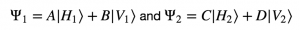
To illustrate how an entangled state differs from a simple superposition of two states, we can consider two photons that have two corresponding polarization states, horizontal or vertical. A non-entangled state for each photon would look like the following:

[1]

In this case, each photon is in a superposition of vertical and horizontal polarization and the coefficients A,B,C, and D represent the probability of measuring vertical or horizontal for each photon.

If the photons were in an entangled state, their wavefunctions could look something like this:

[2]

In this case, both the photons have the same wavefunction, which depends on the horizontal/vertical polarization state of either photon. This means that any measurement of one photon will depend on the measurement of the other. Note that there are multiple ways to achieve this; the equation above is just one example.

To illustrate this further, we can calculate the expectation value of some measurement, by assuming there exists some hermitian operator, O, for this measurement:

If the photons were not entangled:

[3]

If the photons were entangled,

[4]

Equation 3 shows that the non-entangled photon has an expectation value for the measurement that only depends on its own polarization state. In contrast, equation 4 shows that this expectation value for an entangled particle depends on the polarization states of both particles. Thus, at the time of the measurement, both particles will instantaneously collapse into corresponding states.

Hidden Variable Theory

We can also examine entanglement through the lens of hidden variable theory. As stated above, when one measurement is taken from a member of an entangled pair, the other one instantaneously collapses into a corresponding state based on their mutually dependent wavefunction. Even if the photons are on opposite ends of the universe, this collapsing effect would theoretically be the same. If the wavefunctions collapse instantaneously even at astronomical distances, then information needs to travel faster than the speed of light. One explanation for this “magical” phenomenon is that there exist hidden variables that predetermine the outcome of each measurement before it occurs.

In 1969, Clauser, Horne, Shimony, and Hotle (CHSH) created a generalized hidden variable theory which they used to derive an inequality that would only be true if hidden variables are at play in a given measurement. [2] They did this by assuming the outcome of a given measurement depends on the independent parameters involved and some arbitrary “hidden variable” in some way. Then, they derive an expression, Bell’s inequality, which will always be true for a given set of measurements if hidden variables are involved. The derivation of this inequality is not trivial and purely mathematical, so it is not relevant to this project. They also proposed an experiment to test their inequality that consists of measuring the number of coincident photons as a function of polarization of either photon. If we can prove that no hidden variables exist, then we will show that the behavior of entangled particles contradicts our understanding of classical physics.

Testing Quantum Entanglement Experimentally

To conduct our entanglement experiment, we utilized the phenomenon of spontaneous parametric down-conversion (SPDC). SPDC occurs when light passes through a nonlinear crystal (in our case BBO). A small number of photons that pass through the crystal split into two photons with equal energy that is half that of the incoming photons. They also have the same polarization that is orthogonal to the polarization of the incident photon due to conservation of angular momentum.  In our experiment, we sent a purple laser first through a half-wave plate to polarize the laser light at 45 degrees. The polarized laser light then passed through two BBO crystals oriented perpendicular to each other. This means that the down-converted photons could either be horizontally or vertically polarized, but since we can’t predict which crystal produced the pair, we don’t know their polarization. This phenomenon causes the photons to be in an entangled state, where the measured polarization of one photon depends on that of the other.  If the photons were not entangled, they would be in a randomly mixed state of horizontal and vertical polarization, whereas entangled photon pairs would have correlated polarizations.

The following formulas define variables, E and S, which don’t have a physical meaning. These formulas are just CSHC’s original hidden variable theory rearranged in a more convenient manner.[1][3]

[5]

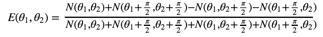
 [6]

In these formulas, N is the number of coincidences recorded for the given combination of polarizer angles. Theta1 and theta1 prime are any two polarization and angles for detector A and theta2 and theta2 prime are any two polarization angles for detector B. Based on the work of CHSH S ≤ 2 if hidden variables are involved in the measurement of coincidences.[1][3] Thus, the expected results of our experiment would be an S that is greater than 2.

Experimental Procedure

Figures 1 and 2 show our experimental setup. The laser is shot through the half-wave plate, the BBO crystals, and also a quartz that corrects for the phase shift of the laser light.

We can see that the two detectors on the other side of the optical table are approximately equidistant from the principle beam in order to detect the two streams of down-converted photons. There is a polarizer in front of each detector in order for us to test the CHSH hidden variable theory. We also placed infrared filters in front of each detector so that they would only detect the stream of infrared photons.

Figure 1: Birds-eye view of experimental setup

Figure 1: Close up of detectors with polarizers in front

We used a LabView program (made by previous Vassar students) to record the total number of coincidences in each a 10 second interval. A coincidence is recorded every time the detectors register a photon instantaneously. Since the down-converted photons are in an entangled polarization state and have correlated polarization, the number of coincidences is a function of polarizer angle. The number of coincidences is also the measurement needed to verify equations 5 and 6.

Since S depends on configurations independent calculation of E, and each calculation of E depends on the number of coincidences at four polarizer configurations, we needed to measure the number of coincidences at 16 polarizer configurations in total.

Results and Conclusions

Table 1 shows the results of our experiment. The number of coincidences is clearly a function of polarizer angle, which indicates that the photons are in fact in an entangled state.

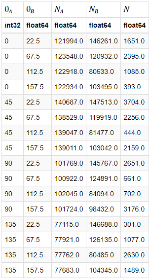
Table 1: Coincidence counts and total counts in each detector at each of the 16 combinations of polarizer angles. The first two columns show the angle of each polarizer. The third column shows the counts in detector A, the fourth shows the counts in detector B, and the fifth shows the coincidence counts.

Our final value of S, using equations 5 and 6 was -0.0465±0.0396. Unfortunately, this obeys Bell’s inequality for hidden variables, which is the opposite of what we had expected. We know from many previous repetitions of this experiment at other institutions, that Bell’s inequality should not hold in this experiment.[1][3] The uncertainty in our value of S is also about the same as the calculated value itself, so we are not very confident in our result.

There are various sources of error that could have resulted in the data we collected. There could have been some sort of light pollution that we weren’t accounting for or some hardware error. However, since our experimental setup has been extensively tested by previous students, these effects probably weren’t significant enough for us to get such an inaccurate value of S.

The most likely cause of the discrepancy between our data and the CHSH theory is improper alignment. Most of our time working on this project was spent attempting to align the laser. We struggled not only to align the detector with the beam infrared photons, but also to maximize the coincidences. For a more detailed description of our struggles, see Jay’s project.

From comparing our data to the data collected by Dehlinger and Mitchell using a similar experimental setup[1], we have deduced that at a given polarizer angle for detector A, the number of coincidences should vary sinusoidally with the polarizer angle for detector B. Figure 3 shows that at the different values of angle for polarizer A, the number of coincidences does not vary in this fashion with the angle for polarizer B.  We think that we could solve this issue by aligning the two detectors more thoroughly. The down-converted photons are actually emitted in ring, where photons across from each other are entangled pairs (illustrated in Figure 4). This means that if our detectors weren’t on the exact spots on the ring that correspond to an entangled pair, our data would not necessarily be consistent with CHSH theory or previous results. For future research, if we were able to place both detectors in some sort of circular mount with adjustable positions, then we would be able to more easily identify these exact positions. We also began our experiment with detector A already aligned and proceeded to align detector B. It is possible that we would have needed to align detector A more exactly in order to locate the correct ring positions.

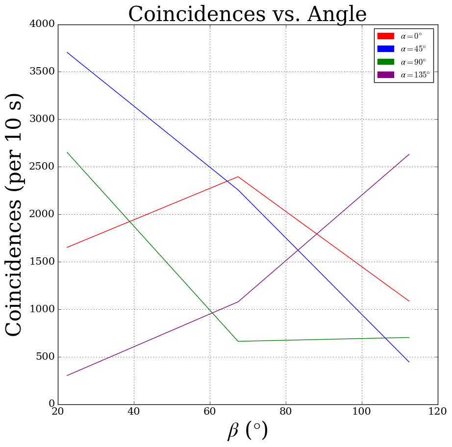
Figure 4: Number of coincidences as a function of polarizer angle for detector B (beta) at different values of polarizer angle for detector A (alpha).

 

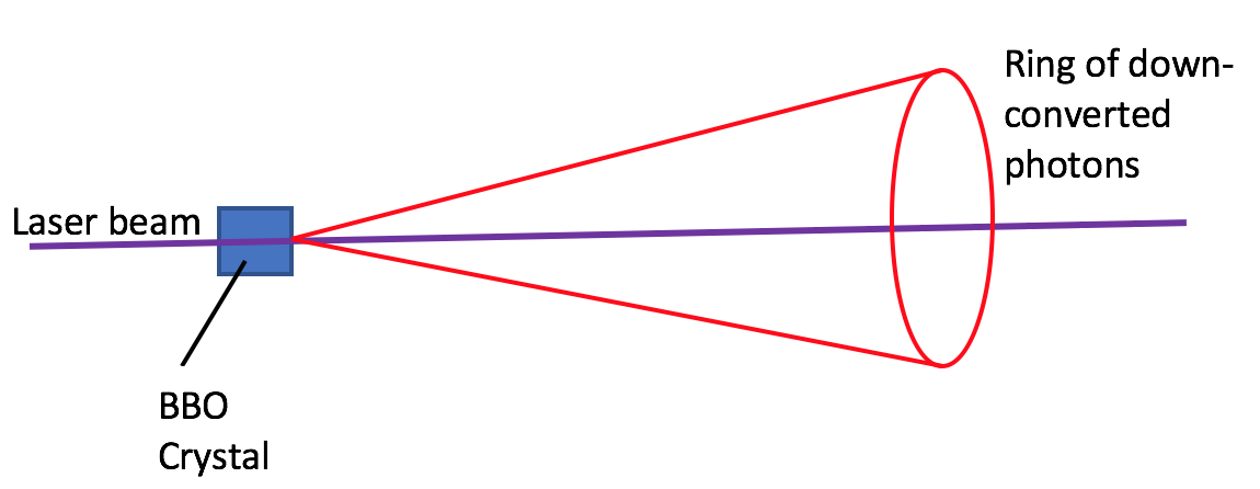
Figure 5: Schematic of SPDC. The entangled pairs are emitted in all orientations but at the same angle. They end up emerging from the BBO crystal in a ring shape, with entangled pairs exactly across from each other.

Regardless of some clear experimental issues, we were able to observe quantum entanglement in action. Although the number of coincidences we recorded did not show the correct dependance on polarizer angle, they displayed a clear relationship. This is a clear indicator that when one member of an entangled pair is counted, the other must instantaneously collapse into a corresponding polarization state to be counted by the other detector. And although we did not end up disproving CHSH’s hidden variable theory, our calculation of S came with an unreasonable uncertainty, so our results cannot prove that hidden variables exist. Inconclusive results aside, this project was very useful in illustrating the concepts of quantum entanglement and hidden variables, which relate to the most fundamental concepts of quantum mechanics such as superposition and deviation from classical mechanics. If anything, this experiment allows us to observe the oddity of quantum mechanics by simply counting photons.

References

[1] Dehlinger, Dietrich and Mitchell, M.W. “Entangled photons, nonlocality and Bell inequalities in the undergraduate laboratory.” American Journal of Physics 70, 903 (2002).

[2] John F. Clauser, Michael A. Horne, Abner Shimony, and Richard A. Holt. “Proposed Experiment to Test Local Hidden-Variable Theories” Physics Review Letters 23, 880 (1969).

[3] Galvez, Enrique J. “Correlated Photon Experiments for Undergraduate Labs” Colgate University (2010).