Overview:

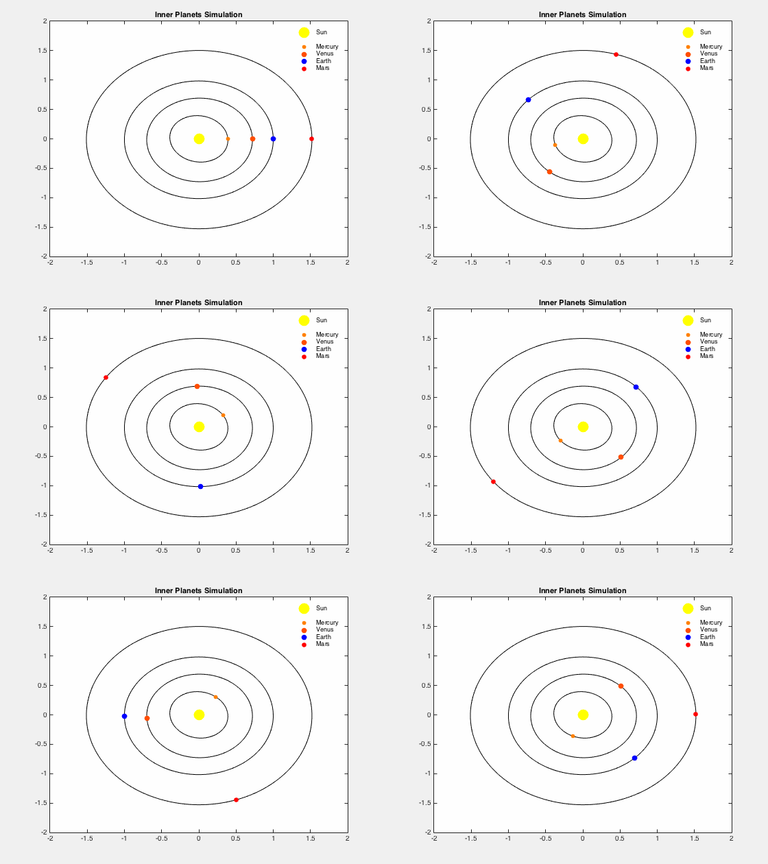
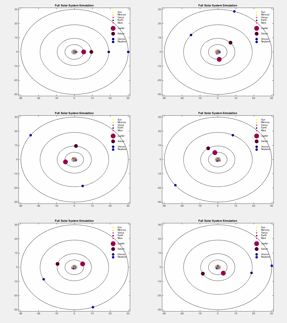
For my final project, I made two animations that model the orbital motion of planets in our solar system based on data sets that I generated. The first animation shows the orbit of the inner planets and the second shows the full solar system. While the spacing of the planets is to scale, the size of the planets is not. The sun and eight planets are simulated in two-dimensional plots with the sun at the origin (sorry Pluto!). The plots are in the reference frame of the sun, so the sun is at rest. The planets are color-coded based on the dominant color of their surface (i.e. yellow for the sun, red for Mars, etc). The full orbital paths are shown in the plots along with the moving planets for reference. The plots show at least one full revolution for each planet. This program was created for educational purposes. My intentions are that this program could be shown to children learning about the solar system to give them an idea of the scale of the solar system relative to Earth and a visual representation of the difference in orbital periods.

Background, Methods, and Assumptions:

The data sets were generated using the Euler-Cromer method. I made several key simplifying assumptions that led to the model I used. I assumed that the sun is exactly centered in each planet’s orbit. I assumed that the effects of gravity were only between an individual planet and the sun, with planets having no effect on each other. By also assuming the orbits are circular, we equate the centripetal force to the force of gravity to get a zero net force. Using units of AU, we get that the gravitational constant G, multiplied by the mass of the sun, Ms, is equal to 4π². Solving the equation then gives us the following equations to calculate the x and y components of the position and velocity for a planet of mass M:

As both the centripetal force equation and gravity force equation have the planet’s mass involved, the final equations surprisingly do not end up involving a factor of the mass. The use of the Euler-Cromer method comes in to play for the position equations, where the velocity calculated for time i+1 is used instead of the velocity from time i (the previous time, as would be used in the Euler method).  I initialized the positions of the planets to be at their respective average distance from the sun along the x-axis. The initial velocity at this point of the orbit is completely in the y-direction. It was calculated by dividing the circumference (still assuming a circular orbit) by the period in terms of an Earth year (for Earth, the initial velocity was 2π AU/Earth year). Based on these initial conditions, I looped through the equations over a time window of 300 with a time step of .005 to generate my data. This process was repeated for each planet using essentially the same code but with different initial positions and velocities. Once I had my data calculated, all that was left was to plot. The orbits calculated are not consistent as the planets make successive revolutions about the sun, resulting in an overlapping ellipse pattern when the full data set was plotted. I plotted a section of the data for each planet that included one orbit to show the path. The for loops plotted one position pair at a time successively, resulting in the animated planets orbiting the stationary sun.

Visualizations:

Inner Planets Simulation

Full Solar System Simulation

 

Results

As I was trying to model an existing system, I had information to compare my results with. The main way I judged the effectiveness of the program is the relative orbital periods of the planets. The real orbital periods compared to Earth are shown in the following table:

Planet	Approximate Earth orbits per one orbit
Mercury	.24
Venus	.62
Earth	1
Mars	1.9
Jupiter	11.9
Saturn	29.4
Uranus	83.7
Neptune	163.7

For one Earth period, Mercury should undergo about four and an eighth periods and Venus should have one and two-thirds periods. Using somewhat qualitative observations by tracking the planets in the animations, I found that my program has very accurate relative orbits as compared to the exact data. My orbits are, however, seem more elliptical than they should be.

 

Discussion:

A number of the simplifying assumptions made are blatantly not correct. The assumption made that the orbits are circular is not true, especially for Mercury, which has a higher eccentricity. I found it quite interesting that, despite creating the model around circular orbits, the calculated orbits ended up being elliptical. Assuming that the sun is centered in the orbits is wrong, as Kepler’s laws state the sun should be at one focus of the orbit. As the orbits are not actually circular, this means that the sun would not be centered (although most planets have a low eccentricity so this would be only a small shift). The time step used must be quite small, or else the orbits will break down (this happens very quickly for Mercury as the time step is increased). I made the decision to have two animations in order for the inner planet orbits to be clearly observable. In the full solar system plot, it is clear that the periods of the smaller planets run much shorter than the outer planets. Apart from that fact, little else can be seen regarding those orbits due to the scale of Neptune’s distance from the sun. The length of Neptune’s period compared to the rest of the planets created other issues as well. The animations themselves take a long time to run, which is somewhat necessary to have a complete cycle for Neptune.  Another limitation is the amount of computation used in the animations. I ended up using 32 vectors with 60000 entries each to hold all the data, along with several other variables to hold enough information to track a full revolution for Neptune. The visualizations lack legends when the code is run. When legends are included in the plots, the time between frames in the animation was reset from what I coded it to be and the animation slowed down substantially. For this reason the code for legends was commented out in the Matlab program (it can be uncommented if legends are desired at the user’s risk of very long runtimes for the animations). For the visualizations, I was able to override the time in between images in the .gif, and so legends are included in the figures shown.

 

Conclusion:

I was able to successfully and accurately model a somewhat simplified version of our solar system. The Euler-Cromer method was appropriate for this task and I would continue to use it in further investigations. In terms of moving forward with this program, my next steps might be making the program interactive. This process would include allowing the user to select the number of planets, the mass, radii, color, and other parameters. It would also be nice to incorporate moons into the simulation. In terms of improving the current program, I would try to figure out a way to include the legends in the program without disrupting the speed of the animations in the code (this would especially be necessary if the program was interactive). Creating an algorithm to optimize the number of data points needed to have one full period for each planet would also be useful to streamline the data.

 

References:

Giordano, Nicholas J., and Hisao Nakanishi. Computational Physics. 2nd ed. Upper Saddle River, NJ: Prentice Hall, 2006. Print.

“Kepler’s Laws.” HyperPhysics. N.p., n.d. Web. 30 Nov. 2016.

Williams, David R. “Planetary Fact Sheet – U.S. Units.” NASA. NASA, n.d. Web. 20 Nov. 2016.