
My final data builds significantly from the preliminary data sets. In that set, I derived the equations for the electric field of a sphere, cylinder and the approximation of an electric dipole. Those were:
![\[ \textbf{E} = \frac{q_e}{\epsilon_0 4 \pi r^2} \textbf{$\hat{r}$} \]](https://pages.vassar.edu/magnes/wp-content/ql-cache/quicklatex.com-3e809ffe305a5dd257991f875380bb3e_l3.png "Rendered by QuickLaTeX.com")
![\[ \textbf{E} = \frac{\rho R^2 }{2r\epsilon_0} \textbf{$\hat{r}$} \]](https://pages.vassar.edu/magnes/wp-content/ql-cache/quicklatex.com-555b4e970293d3e4e78338dd68259d29_l3.png "Rendered by QuickLaTeX.com")
Where the dipole was approximated as two point charges of opposite charge (i.e. two spheres of opposite charge).
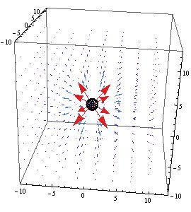
I went back to mathematica and overlaid a 3-D model of a small sphere on the previously plotted vector field of the electric field of a sphere, pictured below.
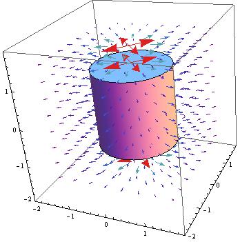
The same was done for a cylinder, both cases allowed for it to be seen how the geometries affected the electric fields.
For the electric dipole, an additional approach was taken to find the electric field. The equation for the electric potential of an “ideal” dipole is given as
![\[ V = \frac{p_o \cos(\theta)}{\epsilon_0 4 \pi r^2} \]](https://pages.vassar.edu/magnes/wp-content/ql-cache/quicklatex.com-e0d3b83684360e0a3e0cfeac94fc47a1_l3.png "Rendered by QuickLaTeX.com")
For the purposes of simplification in Mathematica, the equation was re-written to absorb all the constants into one term:
![\[ V = \frac{p \cos(\theta)}{r^2} \]](https://pages.vassar.edu/magnes/wp-content/ql-cache/quicklatex.com-17a8904c297439b92bb61b4fbb16897e_l3.png "Rendered by QuickLaTeX.com")
Now to find an expression for the electric field, use the formula:
![\[ \textbf{E} = -\nabla V \]](https://pages.vassar.edu/magnes/wp-content/ql-cache/quicklatex.com-4af224d44a6a6606401ab97bc7cbea18_l3.png "Rendered by QuickLaTeX.com")
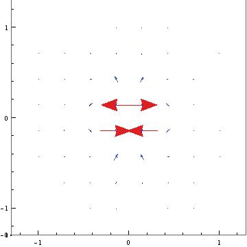
Which Mathematica can interpret and plot accordingly as:

For a better view of how the vectors are interacting, look at this 2-D plot of the same field:
The code for the following models can be found here: Final Data

Don’t forget to label your axis. You need a better way to represent the dipole field. It is unclear what you are modeling and where the charges are located. The spherical vector fields are easily found in Mathematica. Try to come up with a better visualization for the dipole.