Final Data- RLC Circuits

Overview

After talking with Professor Magnes after my preliminary results, I decided to first look at an RLC circuit with no voltage source, which is much simpler to model. Doing this allowed me to better understand the mechanism behind the circuitry and gain more experience with Mathematica as well.

After doing so, I returned to my progress with an RLC circuit with a voltage source and determined that the odd structural variations with the long-term structure were due to computational limitations of Mathematica (again, thanks to Professor Magnes for the suggestion). Since I had only developed the approximate solution, I went on to graphically solve for the full solution and see what the damping terms did to the solution.

Note: I included the findings from my preliminary data in this final data post (so it may seem redundant for a portion in the middle) since it was used in my final results as well. I figured it helps to have everything in one place for the reader.

RLC Circuit with no voltage source

Circuit Diagram and Mathematics

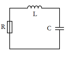
The first circuit we will examine is an RLC circuit with no voltage source. The initial potential difference is stored on the capacitor, but can not be recharged due to the lack of a voltage source. The three main components of this circuit are a resistor (R), an inductor (L), and a capacitor (C).

[Figure 1]

The differential equation that governs this circuit is

$LI''(t)+RI'(t)+\frac{1}{C}I(t)= 0$ [1]

where L is the inductance, R is the resistance, C is the capacitance, I is the current through the circuit (which is the same at all places at one time since this is a series circuit), and t is the time.

Solving the Differential Equation

We can set arbitrary values for R, L, and C since they depend on the specific pieces of equipment themselves:

Inductance= 1 Henry
Resistance= 10 ohms
Capacitance= .1 farads

In Mathematica, the command to solve [1] looks like

$\text{DSolve}\left[\frac{\text{Current}(t)}{\text{Capacitance}}+\text{Inductance} \text{Current}''(t)+\text{Resistance} \text{Current}'(t)=0,\text{Current}(t),t\right]$ [2]

which when solved, yields:

$I(t)= c_1 e^{-8.87298 t}+c_2 e^{-1.12702 t}$ [3]

Completing the Full Solution via Graphical Solving

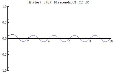
The two constants depend on the initial conditions of the circuit, which must satisfy Ohm’s Law of $I=\frac{V}{R}$ . So, the initial current in the circuit must be 0.1 amps. Using a graphical guess-and-check method in Mathematica, I determined the value of the two constants to be approximately 0.05 each, resulting in a solution that is given by

$I(t)= 0.05 e^{-8.87298 t}+0.05 e^{-1.12702 t}$ [4]

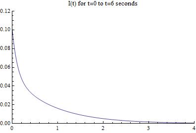
The plot of this equation gives us the current as a function of time, and looks like

[Figure 2]

This graph tells us that although the RLC circuit starts out with a current of 0.1 amps, it quickly dies down due to the lack of a voltage source and is not very interesting after a few seconds. Refer to the upcoming conclusion blog post for a bit more analysis.

Now, lets examine the RLC circuit with a voltage source (much more interesting!)

RLC Circuit with AC voltage source

Circuit Diagram and Mathematics

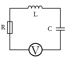
Now we can model an RLC circuit that consists of a capacitor, voltage source, resistor, and an inductor. To easily visualize this, I have constructed a basic circuit diagram (Figure 3).

(Figure 3)

The differential equation that governs this RLC circuit is given by

$LI''(t)+RI'(t)+\frac{1}{C}I(t)= E_{0} \omega cos(\omega t)$ [5]

where L is the inductance, R is the resistance, C is the capacitance, I is the current, $\omega$ is the resonant angular frequency, $E_{0}$ is an initial value dependent on the voltage source, and t is the time. The inductance (L), resistance (R), and capacitance (C)are all determined by their respective circuit components, which are easily changed out for different ones. $\omega$ depends on the inductance and capacitance, and its value is given by

$\omega =\frac{1}{\sqrt{LC}}$ [6]

What we have left in terms of variables are current (I) and time (t). For our purposes, time is the independent variable, which leaves the current in the circuit at any time to be the dependent variable. Now that we have established this, we can solve our differential equation [5] for current as a function of time ( $I(t)$ ).

Solving the Differential Equation

In order to solve [5], I will use the equation solving powers of Mathematica. In particular, the DSolve function is used. When plugged into Mathematica, the input line looks like:

$\text{DSolve}\left[\frac{\text{Current}(t)}{\text{Capacitance}}+\text{Inductance} \text{Current}''(t)+\text{Resistance} \text{Current}'(t)=E_{0} \omega \cos (\omega t),\text{Current}(t),t\right]$ [7]

We must set values for resistance, inductance, capacitance, and $E_{0}$ . For this solution, I chose the same values as the first circuit :

Inductance= 1 Henry
Resistance= 10 ohms
Capacitance= .1 farads
$E_{0}$ = 1 Volt

When the command is run with the above values set, Mathematica generates the general solution, which is:

$I(t)=c_1 e^{-8.87298 t}+c_2 e^{-1.12702 t}+0.040824(-Cos(3.162t)+e^{6.661*10^-16t}Cos(3.162t)-0.3564Sin(3.162t)+2.806e^{6.661*10^-16t}Sin(3.162t))$ [8]

First, lets make sure that this solution is reasonable. The known form of the solution to the equation for such a circuit is given by:

$I(t)=c_1 e^{r_{1}t}+c_2 e^{r_{2}t}+Asin(\omega t-\varphi )$ [9]

The form of our equation [8] seems to match up pretty nicely with this known solution [9]. Now, lets examine [8] in more detail.

Our solution [8] looks a little daunting, but we can break it down into its components. The first two terms have constants that depend on the initial current running through the system, i.e. when $I(t)=I(0)$ . However, we can approximate the equation by only looking at the last term, which is a superposition of sin and cosine functions along with a couple exponential terms thrown in. The reason that we can apply this approximation is that the first two terms “damp out” quickly, and thus have exponentially less of an effect as time progresses. The reader may still be curious to see how much of an effect these terms have on the current flowing through the system: to that I say don’t worry! After my initial approximation, I will solve for these constants and compare the two cases.

Approximate Solution and Graphs

For now, we will deal with the approximate solution, which is:

$I(t)=0.040824(-Cos(3.162t)+e^{6.661*10^-16t}Cos(3.162t)-0.3564Sin(3.162t)+2.806e^{6.661*10^-16t}Sin(3.162t))$ [10]

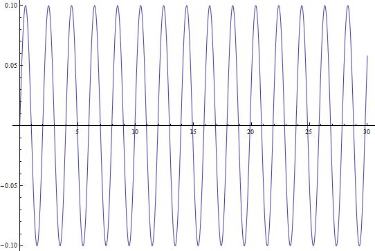
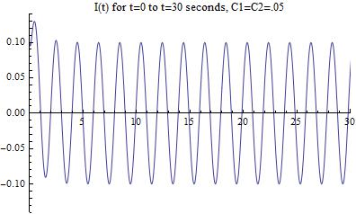
Now that we have this equation, we can use Mathematica to give us an idea of what the changing current looks like over a longer period of time. Figure 2 shows the current in the circuit as a function of time ( $I(t)$ ) plotted over a 30-second interval.

(Figure 4)

This looks like something we would expect! A sinusoidal wave that describes the changing current over time, just like our equations dictate. But, this is a short time-scale. What happens when we look at the changing current over a longer period of time? In Figure 3, I show the changing current over a longer time period (3000 seconds/50 minutes). In Figure 4, I repeat the process, but with the timescale being 5 years.

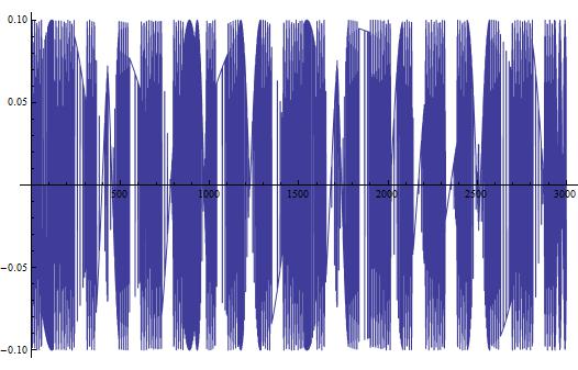(Figure 5)

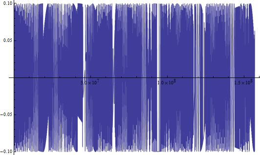(Figure 6)

In both Figures 5 and 6, we see some very interesting long-term variations in the current. Why does this occur?

Computational Limits

It is clear that Mathematica is displaying some odd variations that do not seem to have a set pattern. To investigate this and determine its cause, lets look closer at a range of time where the current seems to be irregular in the previous two figures. Specifically, lets look at the time scale between 300 and 400 seconds because it seems to have very strange behavior.

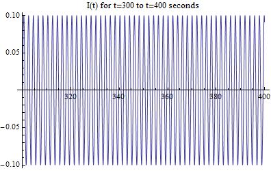[Figure 7]

Looking at the graph above, we see that it looks completely normal! There are no strange variations and the current continues the predicted sinusoidal trend. This leads me to the conclusion that Mathematica has limitations that caused the irregular variations that we saw before, and that they do not actually exist in the data/circuit.

Completing the Full Solution via Graphical Solving

The next and final step in completing our model is accounting for the two initial terms that we left out. Lets take another look at the full equation.

$I(t)=c_1 e^{-8.87298 t}+c_2 e^{-1.12702 t}+0.040824(-Cos(3.162t)+e^{6.661*10^-16t}Cos(3.162t)-0.3564Sin(3.162t)+2.806e^{6.661*10^-16t}Sin(3.162t))$ [11]

We can see that they are exponential functions with a separate constant for each term. Solving for these constants quantitatively can prove to be difficult, so I will attempt to solve for them via a guess-and-check method using plots in Mathematica. I need to match the initial condition so that Ohm’s law is satisfied. So, $I=\frac{V}{R}$ must hold in the initial state. This means that the initial current must be 0.1 amps. Lets try a few values for $C[1]$ and $C[2]$ and figure out graphically what they should be.

First, lets try values of 0.5 for each, resulting in the following equation:

$I(t)=0.5e^{-8.87298 t}+0.5e^{-1.12702 t}+0.040824(-Cos(3.162t)+e^{6.661*10^-16t}Cos(3.162t)-0.3564Sin(3.162t)+2.806e^{6.661*10^-16t}Sin(3.162t))$ [12]

The graph resulting from this equation is:

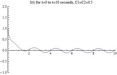[Figure 8]

We can see that the initial current that this combination of constants is too high! It gives 1.0 amps, when we are looking for 0.1 amps.

Lets try slightly higher values for each, as well as having different values for the two. The equation that results is:

$I(t)=2e^{-8.87298 t}+3e^{-1.12702 t}+0.040824(-Cos(3.162t)+e^{6.661*10^-16t}Cos(3.162t)-0.3564Sin(3.162t)+2.806e^{6.661*10^-16t}Sin(3.162t))$ [13]

Which produces the following graph:

[Figure 9]

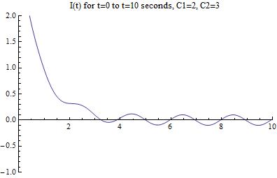
Looks like we have gone the wrong way with our guess! Lets try lowering both the constants to arrive at the correct graphical solution (in reality, this took me many more iterations of guessing and checking):

$I(t)=0.05e^{-8.87298 t}+0.05e^{-1.12702 t}+0.040824(-Cos(3.162t)+e^{6.661*10^-16t}Cos(3.162t)-0.3564Sin(3.162t)+2.806e^{6.661*10^-16t}Sin(3.162t))$ [14]

Which results in the following graph:

[Figure 10]

The Graphical Solution

Now that we have arrived at the correct graphical solution, lets change the scaling of the graph to better match that of [Figure 2], which was the initial approximation that did not take into account the two damping exponential terms.

[Figure 11]

My conclusion from this final data will follow in my next blog post.

Resources

1. Circuit Diagram Maker- http://www.circuit-diagram.org/

2. The RLC Circuit- University of British Columbia- http://www.math.ubc.ca/~feldman/m121/RLC.pdf

3. Mathematica Cookbook by Sal Mangano

4. Electronic Circuit Analysis for Scientists by James A. McCray and Thomas A. Cahill

5. Dynamical Systems with Applications using Mathematica by Stephen Lynch

6. Class Notes- Mathematics 228 (Methods of Applied Mathematics) taught by Matthew Miller

Mathematica Notebook

https://drive.google.com/file/d/0B3mtB6CQNnpjbXROcHl0VURzYlE/edit?usp=sharing

Modeling and Experimental Tools with Prof. Magnes

Ideal for getting ideas and feedback on upper level physics tools.

1 thought on “Final Data- RLC Circuits”