
Overview
In this post, I will draw conclusions from my previous final data post about both RLC circuits that I have modeled.
RLC Circuit- No Voltage Source
This RLC circuit [Figure 1] proved to be an interesting demonstration of the current in a circuit without a voltage source. The initial current running through the circuit is provided by the charged capacitor. However, this initial current undergoes damping due to the resistor in place, and the current running through the circuit pretty approaches zero pretty quickly.
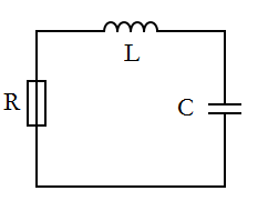 [Figure 1]
My model of this circuit verifies this idea since it shows an exponential decay of the current as a function of time [Figure 2]. After about 4 seconds, there is no longer an active current running through the circuit due to the resistor. My Mathematica notebook is easily set up for changing the values of the different components, and one can easily change them to see what effect this has on the circuit.
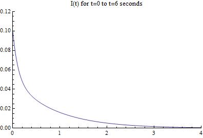 [Figure 2]
RLC Circuit- AC Voltage Source
The second RLC Circuit that I modeled was identical to the one above, except that it had an alternating current voltage source as well [Figure 3]. This allowed it to continue to have a current present despite the effects of the resistor.
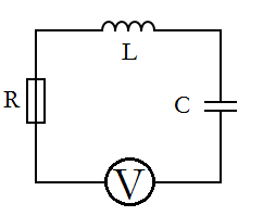 [Figure 3]
Initially, I approximated the solution to the differential equation governing the circuit by ignoring the damping terms. This resulted in a an extremely good approximation, as the damping terms should only effect the circuit’s current flow in its first few seconds. After some computational hiccups that inaccurately displayed long-term variations in the current, I went on to graphically solve the complete form of the equation and graphed it to prove that the two damping terms only had a small effect in the first few seconds of the circuits behavior[Figure 4].
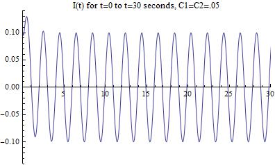 [Figure 4]
Final Remarks
Given the chance to work more on this project, I would develop manipulable animations within Mathematica that would allow one to change a given variable (ex. resistance, inductance, capacitance). This would allow the reader to easily see the effects that the different components have on the circuit. This would also be helpful from an educational standpoint as an applet to someone wanting to learn more about RLC circuits, or circuitry in general.
On a final note, I managed to learn a lot more about Mathematica and its differential equation solving capabilities. Solving the equations for these circuits by hand would have been an extremely length procedure, but once I provided Mathematica with the commands in the correct syntax, it solved them much faster than any human could. This project helped me appreciate the uses of computational tools in physics, and I am very glad that they exist.

Hey Deep!
Great project. I thought your step by step breakdown of your modeling of RLC circuits was very clear. I think this is a wonderful introduction to the mechanism behind such a phenomenon. I have some suggestions on how to improve this project if you were to make it more of a lecture on RLC circuits as a whole, or if you wish to continue your exploration in electronics. It would have been nice to explain all the variables in detail from the beginning. What is a capacitor? What is inductance? Why should they be in series with each other and a resistor, and what specific applications are they used for? Maybe give some several examples of RLC circuits with different values for different variables, and demonstrate mathematically the role of each variable. If you raised the inductance, how would the voltage change when compared to raising the capacitor? Your project could beautifully lead to a discussion on impedance and how you can use that concept in your modeling. Additionally, it would be cool to solve your equation analytically to demonstrate the power of Mathematica and compare that to your solution. Lastly, real world applications in your conclusion would be nice. What applications require higher capacitors or voltage sources with low resistors, and so on? Are there any advantages for the initial peak before the system settles? Could Mathematica model a basic radio, motor, or filters? How about comparing RLC to RL, LC, or RC circuits? These are just some suggestions, and it would be cool to explore more now that you have experience with the software. Given the short time frame of this project, you did more than I would expect one to accomplish with such a topic anyway.
Overall your project was wonderful to read, and a wonderful introduction to RLC circuits and how to use it in Mathematica. I knew Mathematica could solve equations, but I did not know it could do it for complicated differential equations. That is cool! You did a fantastic job.
Have a great summer!